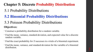
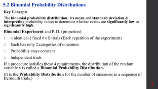
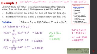
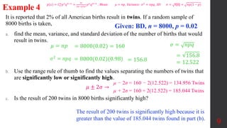
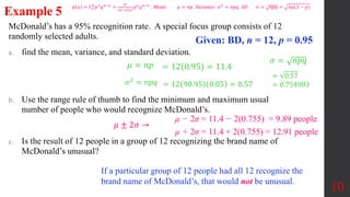
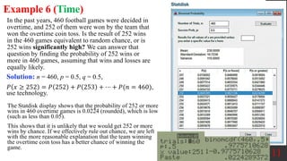
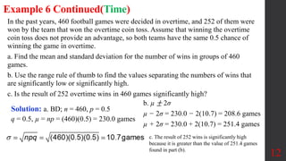
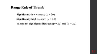
This document discusses the binomial probability distribution, its properties, and how to calculate probabilities, means, variances, and standard deviations for random variables in binomial experiments. It outlines the requirements for a procedure to be classified as a binomial experiment and includes example calculations for various scenarios, such as determining probabilities of certain outcomes. Additionally, it explains how to interpret results based on significance levels and provides guidelines for calculations using statistical tools.

1. Elementary Statistics
Chapter 5:
Discrete Probability
Distribution
5.2 Binomial
Probability
Distribution
1

2. Chapter 5: Discrete Probability Distribution
5.1 Probability Distributions
5.2 Binomial Probability Distributions
5.3 Poisson Probability Distributions
2
Objectives:
• Construct a probability distribution for a random variable.
• Find the mean, variance, standard deviation, and expected value for a discrete
random variable.
• Find the exact probability for X successes in n trials of a binomial experiment.
• Find the mean, variance, and standard deviation for the variable of a binomial
distribution.

3. Key Concept:
The binomial probability distribution, its mean and standard deviation &
interpreting probability values to determine whether events are significantly low or
significantly high.
Binomial Experiment and P. D. (properties)
1. n identical ( fixed # of) trials (Each repetition of the experiment)
2. Each has only 2 categories of outcomes
3. Probability stays constant
4. Independent trials
If a procedure satisfies these 4 requirements, the distribution of the random
variable x is called a Binomial Probability Distribution.
(It is the Probability Distribution for the number of successes in a sequence of
Bernoulli trials.)
5.2 Binomial Probability Distributions
3

4. p = probability of success, q = 1 − p = probability of failure
Make sure that the values of p and x refer to the same category called a success (x and p are consistent).
x: A specific number of successes in n trials: 0 ≤ 𝑥(𝑎 𝑤ℎ𝑜𝑙𝑒 #) ≤ 𝑛
P(x): probability of getting exactly x successes among the n trials
The word success as used here is arbitrary and does not necessarily represent something good. Either of the two
possible categories may be called the success S as long as its probability is identified as p.
Parameters: n & p
Binomial Coefficient (# of outcomes containing exactly x successes): 𝐶𝑥
𝑛
Each trial is known as a Bernoulli trial (named after Swiss mathematician Jacob Bernoulli).
Notes: If the probability of x success in n trials is less than 0.05, it is considered unusual.
5% Guideline for Cumbersome Calculations: When sampling without replacement and the sample size is no
more than 5% of the size of the population, treat the selections as being independent (even though they are
actually dependent).
Warning: If we toss a coin 1000 times, P (H=501), or any specific number of heads is very small, however, we
expect P (at least 501 heads) to be high.
5.2 Binomial Probability Distributions 𝑝(𝑥) = 𝐶𝑥
𝑛
𝑝𝑥
𝑞𝑛−𝑥
4

5. The Probability Histogram is Symmetric if: p = 0.5
The Probability Histogram is Right Skewed: p < 0.5
The Probability Histogram is Left Skewed: p > 0.5
In a binomial experiment, the probability of exactly X successes in n trials is
5.2 Binomial Probability Distributions
𝑃(𝑥) =
𝑛!
(𝑛 − 𝑥)! 𝑥!
⋅ 𝑝𝑥
⋅ 𝑞𝑛−𝑥
Or 𝑃(𝑥) = 𝑛𝐶𝑥
number of possible
desired outcomes
⋅ 𝑝𝑋 ⋅ 𝑞𝑛−𝑋
probability of a
desired outcome
5
𝑝(𝑥) = 𝐶𝑥
𝑛
𝑝𝑥
𝑞𝑛−𝑥
Mean: 𝜇 = 𝑛𝑝
Variance: 𝜎2 = 𝑛𝑝𝑞
SD: 𝜎 = 𝑛𝑝𝑞
= 𝑛𝑝(1 − 𝑝)

6. When an adult is randomly selected (with replacement), there is a 0.85
probability that this person knows what Twitter is. Suppose that we want
to find the probability that exactly three of five randomly selected adults
know what Twitter is.
a. Does this procedure result in a binomial distribution?
b. If this procedure does result in a binomial distribution, identify the
values of n, x, p, and q.
Example 1
a. Solution: Yes
1. Number of trials: n = 5 (fixed)
3. 2 categories: The selected person knows what Twitter is or does not.
4. Constant probability: For each randomly selected adult: x = 3, p =
0.85 & q= 0.15
5. Independent: Different adults (All 5 trials are independent because
the probability of any adult knowing Twitter is not affected by
results from other selected adults.)
6
𝑝 𝑥 = 𝐶𝑥
𝑛
𝑝𝑥
𝑞𝑛−𝑥
=
𝑛!
𝑛−𝑥 !𝑥!
𝑝𝑥
𝑞𝑛−𝑥
, Mean: 𝜇 = 𝑛𝑝, Variance: 𝜎2
= 𝑛𝑝𝑞, SD: 𝜎 = 𝑛𝑝𝑞 = 𝑛𝑝(1 − 𝑝)
b. n = 5, x = 3, p = 0.85, q = 1 − 𝑝 = 0.15
𝑃(3) =
5!
(5 − 3)! 3!
⋅ 0.853 ⋅ 0.155−3 = 10(0.614125)(0.0225)
= 0.1382
TI Calculator:
Binomial Distribution
1. 2nd + VARS
2. Binompdf (
3. Enter: n, p, x
4. Enter
5. If you enter n, p only
6. Gives all probabilities
from 0 to n
7. If using Binomcdf (
8. Gives sum of the
probabilities from 0 to x.
Binomial Experiment and P. D.
(properties)
1. n identical (fixed # of) trials
(Each repetition of the experiment)
2. Each has only 2 categories of
outcomes
3. Probability stays constant
4. Independent trials

7. Assume one out of five people has visited a doctor in any given month. If 10
people are selected at random,
a. find the probability that exactly 3 have visited a doctor last month.
b. find the probability that at most 2 have visited a doctor last month.
c. find the probability that at least 3 have visited a doctor last month.
7
Example 2
Solution
𝐵𝐷: 𝑛 = 10, 𝑝 =
1
5
, 𝑥 = 3
a. 𝑃(3) =
10!
7!3!
1
5
3
⋅
4
5
7
= 0.20133
𝑃(𝑥) =
10!
𝑥! (10 − 𝑥)!
⋅ (1/5)𝑥 ⋅ (4/5)10−𝑥
q = 1 − 𝑝 =
4
5
TI Calculator:
Binomial Distribution
1. 2nd + VARS
2. Binompdf (
3. Enter: n, p, x
4. Enter
5. If you enter n, p only
6. Gives all probabilities
from 0 to n
7. If using Binomcdf (
8. Gives sum of the
probabilities from 0 to x.
b. 𝑃(at most 2) = 𝑃(𝑥 ≤ 2)
c. 𝑃(at least 3) = 𝑃(𝑥 ≥ 3)
𝑃 0 + 𝑃 1 + 𝑃 2
= 1 − 𝑃(𝑥 ≤ 2)
= 0.3222
𝑝 𝑥 = 𝐶𝑥
𝑛
𝑝𝑥
𝑞𝑛−𝑥
=
𝑛!
𝑛−𝑥 !𝑥!
𝑝𝑥
𝑞𝑛−𝑥
, Mean: 𝜇 = 𝑛𝑝, Variance: 𝜎2
= 𝑛𝑝𝑞, SD: 𝜎 = 𝑛𝑝𝑞 = 𝑛𝑝(1 − 𝑝)

8. A survey found that 30% of teenage consumers receive their spending
money from part-time jobs. If 5 teenagers are selected at random,
a. find the probability that at least 3 of them will have part-time jobs.
b. find the probability that at most 2 of them will have part-time jobs.
8
Example 3
Solution 𝐵𝐷: 𝑛 = 5, 𝑝 = 0.30, "at least 3" → 𝑋 = 3,4,5
𝑃(3) =
5!
2! 3!
⋅ 0. 33 ⋅ 0. 72
𝑃(4) =
5!
1! 4!
⋅ 0. 34 ⋅ 0. 71
= 0.1323 𝑃(𝑥 ≥ 3) =
𝐴𝑑𝑑
= 0.16308
= 0.02835
𝑃(5) =
5!
0! 5!
⋅ 0.035 ⋅ 0. 70
= 0.00243
𝑎. 𝑃(at least 3) = 𝑃(𝑥 ≥ 3)
𝑏. 𝑃(𝑥 ≤ 2) =
1 − 𝑃(𝑥 ≥ 3)
= 1 − 0.16308
= 0.83692
TI Calculator:
Binomial Distribution
1. 2nd + VARS
2. Binompdf (
3. Enter: n, p, x
4. Enter
5. If you enter n, p only
6. Gives all probabilities
from 0 to n
7. If using Binomcdf (
8. Gives sum of the
probabilities from 0 to x.
𝑝 𝑥 = 𝐶𝑥
𝑛
𝑝𝑥
𝑞𝑛−𝑥
=
𝑛!
𝑛−𝑥 !𝑥!
𝑝𝑥
𝑞𝑛−𝑥
, Mean: 𝜇 = 𝑛𝑝, Variance: 𝜎2
= 𝑛𝑝𝑞, SD: 𝜎 = 𝑛𝑝𝑞 = 𝑛𝑝(1 − 𝑝)

9. It is reported that 2% of all American births result in twins. If a random sample of
8000 births is taken,
a. find the mean, variance, and standard deviation of the number of births that would
result in twins.
b. Use the range rule of thumb to find the values separating the numbers of twins that
are significantly low or significantly high.
c. Is the result of 200 twins in 8000 births significantly high?
9
Example 4
Given: BD, n = 8000, p = 0.02
𝜇 = 𝑛𝑝
𝜎2 = 𝑛𝑝𝑞
𝜎 = 𝑛𝑝𝑞
= 8000(0.02) = 160
= 8000(0.02)(0.98)
= 156.8
= 12.522
= 156.8
µ − 2σ = 160 − 2(12.522) = 134.956 Twins
µ + 2σ = 160 + 2(12.522) = 185.044 Twins
𝜇 ± 2𝜎 →
The result of 200 twins is significantly high because it is
greater than the value of 185.044 twins found in part (b).
𝑝 𝑥 = 𝐶𝑥
𝑛
𝑝𝑥
𝑞𝑛−𝑥
=
𝑛!
𝑛−𝑥 !𝑥!
𝑝𝑥
𝑞𝑛−𝑥
, Mean: 𝜇 = 𝑛𝑝, Variance: 𝜎2
= 𝑛𝑝𝑞, SD: 𝜎 = 𝑛𝑝𝑞 = 𝑛𝑝(1 − 𝑝)

10. McDonald’s has a 95% recognition rate. A special focus group consists of 12
randomly selected adults.
a. find the mean, variance, and standard deviation.
b. Use the range rule of thumb to find the minimum and maximum usual
number of people who would recognize McDonald’s.
c. Is the result of 12 people in a group of 12 recognizing the brand name of
McDonald’s unusual?
10
Example 5
Given: BD, n = 12, p = 0.95
𝜇 = 𝑛𝑝 = 12(0.95) = 11.4
𝜎2 = 𝑛𝑝𝑞 = 12 90.95 0.05 = 0.57
𝜎 = 𝑛𝑝𝑞
= 0.57
= 0.754983
µ − 2σ = 11.4 − 2(0.755) = 9.89 people
µ + 2σ = 11.4 + 2(0.755) = 12.91 people
𝜇 ± 2𝜎 →
If a particular group of 12 people had all 12 recognize the
brand name of McDonald’s, that would not be unusual.
𝑝 𝑥 = 𝐶𝑥
𝑛
𝑝𝑥
𝑞𝑛−𝑥
=
𝑛!
𝑛−𝑥 !𝑥!
𝑝𝑥
𝑞𝑛−𝑥
, Mean: 𝜇 = 𝑛𝑝, Variance: 𝜎2
= 𝑛𝑝𝑞, SD: 𝜎 = 𝑛𝑝𝑞 = 𝑛𝑝(1 − 𝑝)

11. In the past years, 460 football games were decided in
overtime, and 252 of them were won by the team that
won the overtime coin toss. Is the result of 252 wins
in the 460 games equivalent to random chance, or is
252 wins significantly high? We can answer that
question by finding the probability of 252 wins or
more in 460 games, assuming that wins and losses are
equally likely.
11
Example 6 (Time)
Solution: n = 460, p = 0.5, q = 0.5,
𝑃 𝑥 ≥ 252 = 𝑃 252 + 𝑃 253 + ⋯ + 𝑃(𝑛 = 460),
use technology.
The Statdisk display shows that the probability of 252 or more
wins in 460 overtime games is 0.0224 (rounded), which is low
(such as less than 0.05).
This shows that it is unlikely that we would get 252 or more
wins by chance. If we effectively rule out chance, we are left
with the more reasonable explanation that the team winning
the overtime coin toss has a better chance of winning the
game.

12. In the past years, 460 football games were decided in overtime, and 252 of them were
won by the team that won the overtime coin toss. Assume that winning the overtime
coin toss does not provide an advantage, so both teams have the same 0.5 chance of
winning the game in overtime.
a. Find the mean and standard deviation for the number of wins in groups of 460
games.
b. Use the range rule of thumb to find the values separating the numbers of wins that
are significantly low or significantly high.
c. Is the result of 252 overtime wins in 460 games significantly high?
12
Example 6 Continued(Time)
Solution: a. BD; n = 460, p = 0.5
q = 0.5, µ = np = (460)(0.5) = 230.0 games
b. µ ± 2σ
µ − 2σ = 230.0 − 2(10.7) = 208.6 games
µ + 2σ = 230.0 + 2(10.7) = 251.4 games
c. The result of 252 wins is significantly high
because it is greater than the value of 251.4 games
found in part (b).

13. Range Rule of Thumb
Significantly low values ≤ (µ − 2σ)
Significantly high values ≥ (µ + 2σ)
Values not significant: Between (µ − 2σ) and (µ + 2σ)
13