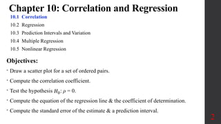
SlideShare a Scribd company logo
1 of 19
Elementary Statistics
Chapter 10: Correlation
and Regression
10.1 Correlation
1
Chapter 10: Correlation and Regression
10.1 Correlation
10.2 Regression
10.3 Prediction Intervals and Variation
10.4 Multiple Regression
10.5 Nonlinear Regression
2
Objectives:
β€’ Draw a scatter plot for a set of ordered pairs.
β€’ Compute the correlation coefficient.
β€’ Test the hypothesis 𝐻0: ρ = 0.
β€’ Compute the equation of the regression line & the coefficient of determination.
β€’ Compute the standard error of the estimate & a prediction interval.
Key Concept: In addition to hypothesis testing and confidence intervals, inferential statistics determines if a
relationship between 2 or more quantitative variables exists.
A correlation exists between two variables when the values of one variable are somehow associated with the
values of the other variable.
A linear correlation exists between two variables when there is a correlation and the plotted points look like a
straight line.
This section considers only linear relationships, which means that when graphed in a scatterplot, the points
approximate a straight-line pattern and methods of conducting a formal hypothesis test that can be used to decide
whether there is a linear correlation between all population values for the two variables.
The linear correlation coefficient r, is a number that measures how well paired sample data fit a straight-line
pattern when graphed (measures the strength of the linear association between the two variables). Use the sample
of paired data (sometimes called bivariate data) to find the value of r, and then use r to decide whether there is a
linear correlation between the two variables.
10.1 Correlation
3
Regression is a statistical method used to describe the nature of the relationship between variablesβ€”that is,
positive or negative, linear or nonlinear.
Questions: 1. Are two or more variables related?
2. If so, what is the strength of the relationship?
3. What type of relationship exists?
4. What kind of predictions can be made from the relationship?
Scatterplots & The Strength of the Linear
Correlation: r
A scatter plot is a graph of the ordered pairs (x, y)
x: the independent variable
y: the dependent variable y.
a. Distinct straight-line, or linear, pattern. We say that there is a
positive linear correlation between x and y, since as the x values
increase, the corresponding y values also increase.
b. Distinct straight-line, or linear pattern. We say that there is a
negative linear correlation between x and y, since as the x values
increase, the corresponding y values decrease.
c. No distinct pattern, which suggests that there is no correlation
between x and y.
d. Distinct pattern suggesting a correlation between x and y, but the
pattern is not that of a straight line.
4
Linear Correlation Coefficient r
1. Are two or more variables related?
2. If so, what is the strength of the relationship?
To answer these two questions, statisticians use the correlation coefficient, a numerical measure to determine
whether two or more variables are related and to determine the strength of the relationship between or among the
variables.
β€’ Linear Correlation Coefficient r
ο‚– The linear correlation coefficient r measures the strength of the linear correlation between the paired quantitative x values and y
values in a sample. It determines whether there is a linear correlation between two variables.
3. What type of relationship exists?
There are two types of relationships: Simple and Multiple
In a simple relationship, there are two variables: an independent variable (predictor variable) and a dependent
variable (response variable).
In a multiple relationship, there are two or more independent variables that are used to predict one dependent
variable.
4. What kind of predictions can be made from the relationship?
Predictions are made daily in all areas. Examples include weather forecasting, stock market analyses, sales
predictions, crop predictions, gasoline price predictions, and sports predictions. Some predictions are more accurate
than others, due to the strength of the relationship. That is, the stronger the relationship is between variables, the
more accurate the prediction is. 5
6
Construct a scatter plot for the data
shown for car rental companies in the
United States for a recent year.
Example 1
Step 1: Draw and label the x and y axes.
Step 2: Plot each point on the graph.
TI Calculator:
Scatter Plot:
1. Press on Y & clear
2. 2nd y (STATPLOT), Enter
3. On, Enter
4. Select X1-list: π‘³πŸ
5. Select Y1-list: π‘³πŸ
6. Mark: Select Character
7. Press Zoom & 9 to get
ZoomStat
TI Calculator:
How to enter data:
1. Stat
2. Edit
3. ClrList π‘³πŸ
4. Or Highlight & Clear
5. Type in your data in L1, ..
Calculating and Interpreting the Linear Correlation Coefficient denoted by r
The correlation coefficient computed from the sample data measures the strength and direction of a linear relationship between two
variables.
There are several types of correlation coefficients. The one explained in this section is called the Pearson product moment correlation
coefficient (PPMC).
The symbol for the sample correlation coefficient is r. The symbol for the population correlation coefficient is .
The range of the correlation coefficient is from ο€­1 to 1.
If there is a strong positive linear relationship between the variables, the value of r will be close to 1. (0.7 or larger)
If there is a strong negative linear relationship between the variables, the value of r will be close to ο€­1. (ο€­ 0.7 or smaller)
n number of pairs of sample data, βˆ‘x = sum of all x’s, βˆ‘xΒ² = Sum of (x values that are squared)
(βˆ‘x)Β² Sum up the x values and square the total. Avoid confusing βˆ‘xΒ² and (βˆ‘x)Β².
βˆ‘xy indicates that each x value should first be multiplied by its corresponding y value. After obtaining all such products, find their
sum.
r linear correlation coefficient for sample data
𝝆 (Rho) : linear correlation coefficient for a population of paired data
7
Given any collection of sample paired quantitative data, the linear correlation coefficient r can
always be computed, but the following requirements should be satisfied when using the sample
paired data to make a conclusion about linear correlation in the corresponding population of
paired data.
1. The sample of paired (x, y) data is a simple random sample of quantitative data.
2. Visual examination of the scatterplot must confirm that the points approximate a straight-line
pattern.
3. Because results can be strongly affected by the presence of outliers, any outliers must be removed if
they are known to be errors. The effects of any other outliers should be considered by calculating r
with and without the outliers included.
4. In other words, requirements 2 and 3 are simplified attempts at checking that the pairs of (x, y) data
have a bivariate normal distribution.
8
π‘Ÿ =
𝑛( π‘₯𝑦) βˆ’ π‘₯ β€’ 𝑦
𝑛( π‘₯
2
) βˆ’ ( π‘₯)2 𝑛( 𝑦
2
) βˆ’ ( 𝑦)2
π‘Ÿ =
(𝑍π‘₯𝑍𝑦)
𝑛 βˆ’ 1
𝒁𝒙 denotes the z score for an individual sample value x
π’π’š denotes the z score for the corresponding sample value y.
Calculating and Interpreting the Linear Correlation Coefficient denoted by r
Example 2: Finding r Using Technology
The table lists five paired data values. Use technology to find the value of the
correlation coefficient r for the data.
Chocolate 5 6 4 4 5
Nobel 6 9 3 2 11
9
Solution:
The value of r will be automatically calculated with
software or a calculator: r = 0.795
Example 3 a: Finding r Using the following Formula
Use this Formula to find the value of the linear
correlation coefficient r for the five pairs of
chocolate/Nobel data listed in the table.
Chocolate 5 6 4 4 5
Nobel 6 9 3 2 11
10
x (Chocolate) y (Nobel) xΒ² yΒ² xy
5 6 25 36 30
6 9 36 81 54
4 3 16 9 12
4 2 16 4 8
5 11 25 121 55
π‘Ÿ =
5(159) βˆ’ 24 β€’ 31
5(118) βˆ’ 242 5(251) βˆ’ 312
=
51
14(294)
= 0.795
π‘Ÿ =
𝑛( π‘₯𝑦) βˆ’ π‘₯ β€’ 𝑦
𝑛( π‘₯
2
) βˆ’ ( π‘₯)2 𝑛( 𝑦
2
) βˆ’ ( 𝑦)2
TI Calculator:
How to enter data:
1. Stat
2. Edit
3. ClrList π‘³πŸ
4. Or Highlight & Clear
5. Type in your data in L1, ..
TI Calculator:
Linear Regression - test
1. Stat
2. Tests
3. LinRegTTest
4. Enter π‘³πŸ & π‘³πŸ
5. Freq = 1
6. Choose β‰ 
7. Calculate
βˆ‘x = 24 βˆ‘y = 31 βˆ‘xΒ² = 118 βˆ‘yΒ² = 251 βˆ‘xy = 159
Use Formula to find the value of the linear correlation coefficient r for the five pairs of
chocolate/Nobel data listed in the table.
Solution: The z scores for all of the chocolate values (see the third column) and the z scores
for all of the Nobel values (see the fourth column) are below. The last column lists the
products zx Β· zy.
x (Chocolate) y (Nobel)
5 6
6 9
4 3
4 2
5 11
blank blank
11
Example 3b: Finding r Using the following Formula
=
3.179746
5 βˆ’ 1
= 0.795
This Formula has the advantage of making
it easier to understand how r works. The
variable x is used for the chocolate values,
and the variable y is used for the Nobel
values. Each sample value is replaced by its
corresponding z score.
For Example:
Chocolates: π‘₯ =
π‘₯
𝑛
= 4.8
𝑠π‘₯ =
(π‘₯ βˆ’ π‘₯)2
𝑛 βˆ’ 1
= 0.836660,
π‘₯ = 5 β†’ 𝑧π‘₯ =
π‘₯ βˆ’ π‘₯
𝑠π‘₯
=
5 βˆ’ 4.8
0.83666
= 0.23905
π‘Ÿ =
(𝑍π‘₯𝑍𝑦)
𝑛 βˆ’ 1
zx zy
0.239046 βˆ’0.052164
1.434274 0.730297
βˆ’0.956183 βˆ’0.834625
βˆ’0.956183 βˆ’1.095445
0.239046 1.251937
zx Β· zy
βˆ’0.012470
1.047446
0.798054
1.047446
0.299270
βˆ‘ (zx Β· zy) =
3.179746
Example 4: Finding r Using the following Formula
Find the correlation coefficient for the given data.
12
Company
Cars x
(in 10,000s)
Income y
(in billions) xy x2
y2
A
B
C
D
E
F
63.0
29.0
20.8
19.1
13.4
8.5
7.0
3.9
2.1
2.8
1.4
1.5
441.00
113.10
43.68
53.48
18.76
12.75
3969.00
841.00
432.64
364.81
179.56
72.25
49.00
15.21
4.41
7.84
1.96
2.25
Ξ£x =
153.8
Ξ£y =
18.7
Ξ£xy =
682.77
Ξ£x2
=
5859.26
Ξ£y2
=
80.67
Ξ£x = 153.8, Ξ£y = 18.7, Ξ£xy = 682.77, Ξ£x2 = 5859.26, Ξ£y2 = 80.67, n = 6
π‘Ÿ =
6(682.77) βˆ’ 153.8 β€’ 18.7
6(5859.26) βˆ’ 153. 82 6(80.67) βˆ’ 18. 72
= 0.982
(strong positive relationship)
π‘Ÿ =
𝑛( π‘₯𝑦) βˆ’ π‘₯ β€’ 𝑦
𝑛( π‘₯
2
) βˆ’ ( π‘₯)2 𝑛( 𝑦
2
) βˆ’ ( 𝑦)2
TI Calculator:
How to enter data:
1. Stat
2. Edit
3. ClrList π‘³πŸ
4. Or Highlight & Clear
5. Type in your data in L1, ..
TI Calculator:
Linear Regression - test
1. Stat
2. Tests
3. LinRegTTest
4. Enter π‘³πŸ & π‘³πŸ
5. Freq = 1
6. Choose β‰ 
7. Calculate
Null Hypothesis: H0: ρ = 0 (No correlation) Alternative Hypothesis: H1: ρ β‰  0 (Correlation)
Using P-Value from Technology to Interpret r:
P-value ≀ Ξ±: Reject 𝐻0 β†’ Supports the claim of a linear correlation.
P-value > Ξ±: Does not support the claim of a linear correlation.
Using Pearson Correlation coefficient table to Interpret r: Consider critical values from
this Table or technology as being both positive and negative:
β€’ Correlation If |r| β‰₯ critical value β‡Ύ There is sufficient evidence to support the claim of a linear
correlation.
β€’ No Correlation If |r| < critical value β‡Ύ There is not sufficient evidence to support the claim of a
linear correlation.
Properties of the Linear Correlation Coefficient r
1. βˆ’1 ≀ r ≀ 1.
2. If all values of either variable are converted to a different scale, the value of r does not change.
4. The value of r is not affected by the choice of x or y. Interchange all x values and y values, and
the value of r will not change. ​​r measures the strength of a linear relationship. It is not designed
to measure the strength of a relationship that is not linear.
5. r is very sensitive to outliers in the sense that a single outlier could dramatically affect its value. 13
Calculating and Interpreting the Linear Correlation Coefficient denoted by r
14
10.1 Correlation
A correlation exists between two variables when the values of one variable are
somehow associated with the values of the other variable. A linear correlation exists
between two variables when there is a correlation and the plotted points look like a
straight line. The linear correlation coefficient r, is a number that measures how well
paired sample data fit a straight-line pattern when graphed (measures the strength of the
linear association between paired data called bivariate data). The value of rΒ² is the
proportion of the variation in y that is explained by the linear relationship between x
and y.
Properties of the Linear Correlation Coefficient r: βˆ’1 ≀ r ≀ 1
zx denotes the z score
for an individual
sample value x
zy is the z score for the
corresponding sample
value y.
𝑇𝑆: 𝑑 = π‘Ÿ
𝑛 βˆ’ 2
1 βˆ’ π‘Ÿ2
=
π‘Ÿ
1 βˆ’ π‘Ÿ2
𝑛 βˆ’ 2
, 𝑑𝑓 = 𝑛 βˆ’ 2
π‘‚π‘Ÿ: π‘Ÿ
π‘Ÿ =
𝑛 π‘₯𝑦 βˆ’ π‘₯ 𝑦
𝑛 π‘₯2 βˆ’ π‘₯ 2 𝑛 𝑦2 βˆ’ 𝑦 2
, π‘‚π‘Ÿ: π‘Ÿ =
(𝑍π‘₯𝑍𝑦)
𝑛 βˆ’ 1
Step 1: H0 :𝜌 = 0, H1: 𝜌 β‰  0 claim
& Tails
Step 2: TS: 𝑑 = π‘Ÿ
π‘›βˆ’2
1βˆ’π‘Ÿ2 , OR: r
Step 3: CV using Ξ± From the
T-table or r-table
Step 4: Make the decision to
a. Reject or not H0
b. The claim is true or false
c. Restate this decision: There is / is
not sufficient evidence to support the
claim that…
There is a linear Correlation If |r|
β‰₯ critical value
There is No Correlation If |r| <
critical value
TI Calculator:
Scatter Plot:
1. Press on Y & clear
2. 2nd y (STATPLOT), Enter
3. On, Enter
4. Select X1-list: π‘³πŸ
5. Select Y1-list: π‘³πŸ
6. Mark: Select Character
7. Press Zoom & 9 to get
ZoomStat
TI Calculator:
Linear Regression – test &
Correlation Coefficient π‘Ÿ
1. Stat
2. Tests
3. LinRegTTest
4. Enter π‘³πŸ & π‘³πŸ
5. Freq = 1
6. Choose β‰ 
7. Calculate
TI Calculator:
How to enter data:
1. Stat
2. Edit
3. ClrList π‘³πŸ
4. Or Highlight & Clear
5. Type in your data in L1, ..
𝑑 =
π‘Ÿβˆ’πœ‡π‘Ÿ
1βˆ’π‘Ÿ2
π‘›βˆ’2
,
πœ‡π‘Ÿ = 0 (πΉπ‘Ÿπ‘œπ‘š H0)
15
Test the significance of the given correlation
coefficient using Ξ± = 0.05, n = 6 and r = 0.982.
Example 5
Decision:
a. Reject H0
b. The claim is
True
c. There is a
significant
relationship
between the 2
variables.
Step 1: H0 , H1, claim & Tails
Step 2: TS Calculate (TS)
Step 3: CV using Ξ±
Step 4: Make the decision to
a. Reject or not H0
b. The claim is true or false
c. Restate this decision: There
is / is not sufficient evidence to
support the claim that…
H0: 𝜌 = 0, H1: 𝜌 β‰  0, claim, 2TT
TS: t-distribution 2nd Method: Pearson Correlation
CV: Ξ± = 0.05,
𝑑𝑓 = 𝑛 βˆ’ 2 = 6 βˆ’ 2 = 4
𝑑 = π‘Ÿ
𝑛 βˆ’ 2
1 βˆ’ π‘Ÿ2 =
π‘Ÿ
1 βˆ’ π‘Ÿ2
𝑛 βˆ’ 2
, 𝑑𝑓 = 𝑛 βˆ’ 2
𝑑 = 0.982
6 βˆ’ 2
1 βˆ’ 0.9822 = 10.3981 TS: π‘Ÿ = 0.982
CV: From Pearson
Correlation Coefficient
table: 𝑛 = 6,Ξ± = 0.05
β†’ 𝑑 = Β±2.776 β†’ π‘Ÿ = Β±0.811
16
Given the value of r = 0.801 for 23 pairs of data regarding chocolate
consumption and numbers of Nobel Laureates, and using a significance level
of 0.05; is there sufficient evidence to support a claim that there is a linear
correlation between chocolate consumption and numbers of Nobel
Laureates?
Example 6
Decision:
a. Reject H0
b. The claim is True
c. There is sufficient evidence to support the
conclusion that for countries, there is a linear
correlation between chocolate consumption
and numbers of Nobel Laureates.
CV: Ξ± = 0.05, 𝑑𝑓 = 𝑛 βˆ’ 2
= 23 βˆ’ 2 = 21
TS: 𝑑 = 0.801
23βˆ’2
1βˆ’0.8012
= 6.1314
TS: π‘Ÿ = 0.801
CV: From Pearson
Correlation coefficient
table: n= 23, Ξ± = 0.05
Interpretation: Although we have found a linear
correlation, it would be absurd to think that eating
more chocolate would help win a Nobel Prize.
β†’ 𝑑 = Β±2.080
Table: r = 0.396 < CV < r = 0.444
Technology: r = 0.413 β†’ π‘Ÿ = Β±0.413
H0: 𝜌 = 0, H1: 𝜌 β‰  0, claim, 2TT
Step 1: H0 , H1, claim & Tails
Step 2: TS Calculate (TS)
Step 3: CV using Ξ±
Step 4: Make the decision to
a. Reject or not H0
b. The claim is true or false
c. Restate this decision: There is
/ is not sufficient evidence to
support the claim that…
𝑑 = π‘Ÿ
𝑛 βˆ’ 2
1 βˆ’ π‘Ÿ2 = 𝑑𝑓 = 𝑛 βˆ’ 2
Interpreting r: Explained Variation
The value of rΒ² , called the coefficient of determination, is the proportion of the
variation in y that is explained by the linear relationship between x and y.
π‘Ÿ2
=
𝐸π‘₯π‘π‘™π‘Žπ‘–π‘›π‘’π‘‘ π‘‰π‘Žπ‘Ÿπ‘–π‘Žπ‘‘π‘–π‘œπ‘›
π‘‡π‘œπ‘‘π‘Žπ‘™ π‘£π‘Žπ‘Ÿπ‘–π‘Žπ‘‘π‘–π‘œπ‘›
Using the 23 pairs of chocolate/Nobel data, we get r = 0.801. What proportion of the
variation in numbers of Nobel Laureates can be explained by the variation in the
consumption of chocolate?
17
Solution
With r = 0.801 we get rΒ² = 0.642.
Interpretation
We conclude that 0.642 (or about 64%) of the variation in numbers of Nobel
Laureates can be explained by the linear relationship between chocolate consumption
and numbers of Nobel Laureates.
This implies that about 36% of the variation in numbers of Nobel Laureates cannot be
explained by rates of chocolate consumption.
When the null hypothesis has been rejected for a specific value, any of the following five possibilities can exist.
1. There is a direct cause-and-effect relationship between the variables. That is, x causes y.
water causes plants to grow, poison causes death, heat causes ice to melt
2. There is a reverse cause-and-effect relationship between the variables. That is, y causes x.
Suppose a researcher believes excessive coffee consumption causes nervousness, but the researcher fails to consider that the
reverse situation may occur. That is, it may be that an extremely nervous person craves coffee to calm his or her nerves.
3. The relationship between the variables may be caused by a third variable.
If a statistician correlated the number of deaths due to drowning and the number of cans of soft drink consumed daily during
the summer, he or she would probably find a significant relationship. However, the soft drink is not necessarily responsible
for the deaths, since both variables may be related to heat and humidity.
4. There may be a complexity of interrelationships among many variables.
A researcher may find a significant relationship between students’ high school grades and college grades. But there probably
are many other variables involved, such as IQ, hours of study, influence of parents, motivation, age, and instructors.
5. The relationship may be coincidental.
A researcher may be able to find a significant relationship between the increase in the number of people who are exercising
and the increase in the number of people who are committing crimes. But common-sense dictates that any relationship
between these two values must be due to coincidence.
10.1 Correlation, Possible Relationships Between Variables
18
Interpreting r with Causation:
Correlation does not imply causality!
We noted previously that we should use common sense when interpreting results.
Clearly, it would be absurd to think that eating more chocolate would help win a
Nobel Prize
19
Common Errors Involving Correlation:
1. Assuming that correlation implies causality
2. Using data based on averages
3. Ignoring the possibility of a nonlinear relationship
Hypotheses If conducting a formal hypothesis test to determine whether there is a significant
linear correlation between two variables, use the following null and alternative hypotheses that
use ρ to represent the linear correlation coefficient of the population:
Null Hypothesis H0: ρ = 0 (No correlation)
Alternative Hypothesis H1: ρ β‰  0 (Correlation)

More Related Content

What's hot

Testing a Claim About a Proportion
Testing a Claim About a ProportionTesting a Claim About a Proportion
Testing a Claim About a ProportionLong Beach City College
Β 
Practice test 3A, Normal Probability Distribution
Practice test 3A, Normal Probability DistributionPractice test 3A, Normal Probability Distribution
Practice test 3A, Normal Probability DistributionLong Beach City College
Β 
Two Variances or Standard Deviations
Two Variances or Standard DeviationsTwo Variances or Standard Deviations
Two Variances or Standard DeviationsLong Beach City College
Β 
Practice test ch 10 correlation reg ch 11 gof ch12 anova
Practice test ch 10 correlation reg ch 11 gof ch12 anovaPractice test ch 10 correlation reg ch 11 gof ch12 anova
Practice test ch 10 correlation reg ch 11 gof ch12 anovaLong Beach City College
Β 
Solution to the practice test ch 8 hypothesis testing ch 9 two populations
Solution to the practice test ch 8 hypothesis testing ch 9 two populationsSolution to the practice test ch 8 hypothesis testing ch 9 two populations
Solution to the practice test ch 8 hypothesis testing ch 9 two populationsLong Beach City College
Β 
Solution to the Practice Test 3A, Chapter 6 Normal Probability Distribution
Solution to the Practice Test 3A, Chapter 6 Normal Probability DistributionSolution to the Practice Test 3A, Chapter 6 Normal Probability Distribution
Solution to the Practice Test 3A, Chapter 6 Normal Probability DistributionLong Beach City College
Β 
Complements and Conditional Probability, and Bayes' Theorem
 Complements and Conditional Probability, and Bayes' Theorem Complements and Conditional Probability, and Bayes' Theorem
Complements and Conditional Probability, and Bayes' TheoremLong Beach City College
Β 
Estimating a Population Standard Deviation or Variance
Estimating a Population Standard Deviation or Variance Estimating a Population Standard Deviation or Variance
Estimating a Population Standard Deviation or Variance Long Beach City College
Β 
Graphs that Enlighten and Graphs that Deceive
Graphs that Enlighten and Graphs that DeceiveGraphs that Enlighten and Graphs that Deceive
Graphs that Enlighten and Graphs that DeceiveLong Beach City College
Β 

What's hot (20)

Assessing Normality
Assessing NormalityAssessing Normality
Assessing Normality
Β 
Testing a Claim About a Proportion
Testing a Claim About a ProportionTesting a Claim About a Proportion
Testing a Claim About a Proportion
Β 
Practice test 3A, Normal Probability Distribution
Practice test 3A, Normal Probability DistributionPractice test 3A, Normal Probability Distribution
Practice test 3A, Normal Probability Distribution
Β 
Probability Distribution
Probability DistributionProbability Distribution
Probability Distribution
Β 
Practice Test 1
Practice Test 1Practice Test 1
Practice Test 1
Β 
Two Variances or Standard Deviations
Two Variances or Standard DeviationsTwo Variances or Standard Deviations
Two Variances or Standard Deviations
Β 
Practice test ch 10 correlation reg ch 11 gof ch12 anova
Practice test ch 10 correlation reg ch 11 gof ch12 anovaPractice test ch 10 correlation reg ch 11 gof ch12 anova
Practice test ch 10 correlation reg ch 11 gof ch12 anova
Β 
Counting
CountingCounting
Counting
Β 
One-Way ANOVA
One-Way ANOVAOne-Way ANOVA
One-Way ANOVA
Β 
Practice Test 2 Probability
Practice Test 2 ProbabilityPractice Test 2 Probability
Practice Test 2 Probability
Β 
Testing a Claim About a Mean
Testing a Claim About a MeanTesting a Claim About a Mean
Testing a Claim About a Mean
Β 
Solution to the practice test ch 8 hypothesis testing ch 9 two populations
Solution to the practice test ch 8 hypothesis testing ch 9 two populationsSolution to the practice test ch 8 hypothesis testing ch 9 two populations
Solution to the practice test ch 8 hypothesis testing ch 9 two populations
Β 
Solution to the Practice Test 3A, Chapter 6 Normal Probability Distribution
Solution to the Practice Test 3A, Chapter 6 Normal Probability DistributionSolution to the Practice Test 3A, Chapter 6 Normal Probability Distribution
Solution to the Practice Test 3A, Chapter 6 Normal Probability Distribution
Β 
Complements and Conditional Probability, and Bayes' Theorem
 Complements and Conditional Probability, and Bayes' Theorem Complements and Conditional Probability, and Bayes' Theorem
Complements and Conditional Probability, and Bayes' Theorem
Β 
The Standard Normal Distribution
The Standard Normal DistributionThe Standard Normal Distribution
The Standard Normal Distribution
Β 
Basic Concepts of Probability
Basic Concepts of ProbabilityBasic Concepts of Probability
Basic Concepts of Probability
Β 
Two Means, Independent Samples
Two Means, Independent SamplesTwo Means, Independent Samples
Two Means, Independent Samples
Β 
Practice Test 1 solutions
Practice Test 1 solutions  Practice Test 1 solutions
Practice Test 1 solutions
Β 
Estimating a Population Standard Deviation or Variance
Estimating a Population Standard Deviation or Variance Estimating a Population Standard Deviation or Variance
Estimating a Population Standard Deviation or Variance
Β 
Graphs that Enlighten and Graphs that Deceive
Graphs that Enlighten and Graphs that DeceiveGraphs that Enlighten and Graphs that Deceive
Graphs that Enlighten and Graphs that Deceive
Β 

Similar to Correlation

Correlation Analysis PRESENTED.pptx
Correlation Analysis PRESENTED.pptxCorrelation Analysis PRESENTED.pptx
Correlation Analysis PRESENTED.pptxHaimanotReta
Β 
Unit 1 Correlation- BSRM.pdf
Unit 1 Correlation- BSRM.pdfUnit 1 Correlation- BSRM.pdf
Unit 1 Correlation- BSRM.pdfRavinandan A P
Β 
Chapter 10
Chapter 10Chapter 10
Chapter 10guest3720ca
Β 
Math n Statistic
Math n StatisticMath n Statistic
Math n StatisticJazmidah Rosle
Β 
Pearson product moment correlation
Pearson product moment correlationPearson product moment correlation
Pearson product moment correlationSharlaine Ruth
Β 
Correlation and Regression
Correlation and Regression Correlation and Regression
Correlation and Regression Dr. Tushar J Bhatt
Β 
Regression
RegressionRegression
RegressionSauravurp
Β 
correlation-analysis.pptx
correlation-analysis.pptxcorrelation-analysis.pptx
correlation-analysis.pptxSoujanyaLk1
Β 
correlation.final.ppt (1).pptx
correlation.final.ppt (1).pptxcorrelation.final.ppt (1).pptx
correlation.final.ppt (1).pptxChieWoo1
Β 
Introduction to correlation and regression analysis
Introduction to correlation and regression analysisIntroduction to correlation and regression analysis
Introduction to correlation and regression analysisFarzad Javidanrad
Β 
Chapter 2 part3-Least-Squares Regression
Chapter 2 part3-Least-Squares RegressionChapter 2 part3-Least-Squares Regression
Chapter 2 part3-Least-Squares Regressionnszakir
Β 
Lecture 13 Regression & Correlation.ppt
Lecture 13 Regression & Correlation.pptLecture 13 Regression & Correlation.ppt
Lecture 13 Regression & Correlation.pptshakirRahman10
Β 
correlation and regression
correlation and regressioncorrelation and regression
correlation and regressionUnsa Shakir
Β 

Similar to Correlation (20)

Correlation Analysis PRESENTED.pptx
Correlation Analysis PRESENTED.pptxCorrelation Analysis PRESENTED.pptx
Correlation Analysis PRESENTED.pptx
Β 
Unit 1 Correlation- BSRM.pdf
Unit 1 Correlation- BSRM.pdfUnit 1 Correlation- BSRM.pdf
Unit 1 Correlation- BSRM.pdf
Β 
Measure of Association
Measure of AssociationMeasure of Association
Measure of Association
Β 
Chapter 10
Chapter 10Chapter 10
Chapter 10
Β 
Chapter 10
Chapter 10Chapter 10
Chapter 10
Β 
Regression
Regression  Regression
Regression
Β 
Chap04 01
Chap04 01Chap04 01
Chap04 01
Β 
Math n Statistic
Math n StatisticMath n Statistic
Math n Statistic
Β 
Pearson product moment correlation
Pearson product moment correlationPearson product moment correlation
Pearson product moment correlation
Β 
Correlation
Correlation  Correlation
Correlation
Β 
Correlation and Regression
Correlation and Regression Correlation and Regression
Correlation and Regression
Β 
Regression
RegressionRegression
Regression
Β 
correlation-analysis.pptx
correlation-analysis.pptxcorrelation-analysis.pptx
correlation-analysis.pptx
Β 
correlation.final.ppt (1).pptx
correlation.final.ppt (1).pptxcorrelation.final.ppt (1).pptx
correlation.final.ppt (1).pptx
Β 
Introduction to correlation and regression analysis
Introduction to correlation and regression analysisIntroduction to correlation and regression analysis
Introduction to correlation and regression analysis
Β 
Chapter 2 part3-Least-Squares Regression
Chapter 2 part3-Least-Squares RegressionChapter 2 part3-Least-Squares Regression
Chapter 2 part3-Least-Squares Regression
Β 
Lecture 13 Regression & Correlation.ppt
Lecture 13 Regression & Correlation.pptLecture 13 Regression & Correlation.ppt
Lecture 13 Regression & Correlation.ppt
Β 
12943625.ppt
12943625.ppt12943625.ppt
12943625.ppt
Β 
Simple lin regress_inference
Simple lin regress_inferenceSimple lin regress_inference
Simple lin regress_inference
Β 
correlation and regression
correlation and regressioncorrelation and regression
correlation and regression
Β 

More from Long Beach City College

More from Long Beach City College (12)

Practice test ch 9 inferences from two samples
Practice test ch 9 inferences from two samplesPractice test ch 9 inferences from two samples
Practice test ch 9 inferences from two samples
Β 
Practice Test Ch 8 Hypothesis Testing
Practice Test Ch 8 Hypothesis TestingPractice Test Ch 8 Hypothesis Testing
Practice Test Ch 8 Hypothesis Testing
Β 
Practice Test Chapter 6 (Normal Probability Distributions)
Practice Test Chapter 6 (Normal Probability Distributions)Practice Test Chapter 6 (Normal Probability Distributions)
Practice Test Chapter 6 (Normal Probability Distributions)
Β 
Stat sample test ch 12 solution
Stat sample test ch 12 solutionStat sample test ch 12 solution
Stat sample test ch 12 solution
Β 
Stat sample test ch 12
Stat sample test ch 12Stat sample test ch 12
Stat sample test ch 12
Β 
Stat sample test ch 11
Stat sample test ch 11Stat sample test ch 11
Stat sample test ch 11
Β 
Stat sample test ch 10
Stat sample test ch 10Stat sample test ch 10
Stat sample test ch 10
Β 
Two-Way ANOVA
Two-Way ANOVATwo-Way ANOVA
Two-Way ANOVA
Β 
Contingency Tables
Contingency TablesContingency Tables
Contingency Tables
Β 
Two Means, Two Dependent Samples, Matched Pairs
Two Means, Two Dependent Samples, Matched PairsTwo Means, Two Dependent Samples, Matched Pairs
Two Means, Two Dependent Samples, Matched Pairs
Β 
Inferences about Two Proportions
 Inferences about Two Proportions Inferences about Two Proportions
Inferences about Two Proportions
Β 
Testing a Claim About a Standard Deviation or Variance
Testing a Claim About a Standard Deviation or VarianceTesting a Claim About a Standard Deviation or Variance
Testing a Claim About a Standard Deviation or Variance
Β 

Recently uploaded

call girls in Kamla Market (DELHI) πŸ” >ΰΌ’9953330565πŸ” genuine Escort Service πŸ”βœ”οΈβœ”οΈ
call girls in Kamla Market (DELHI) πŸ” >ΰΌ’9953330565πŸ” genuine Escort Service πŸ”βœ”οΈβœ”οΈcall girls in Kamla Market (DELHI) πŸ” >ΰΌ’9953330565πŸ” genuine Escort Service πŸ”βœ”οΈβœ”οΈ
call girls in Kamla Market (DELHI) πŸ” >ΰΌ’9953330565πŸ” genuine Escort Service πŸ”βœ”οΈβœ”οΈ9953056974 Low Rate Call Girls In Saket, Delhi NCR
Β 
Difference Between Search & Browse Methods in Odoo 17
Difference Between Search & Browse Methods in Odoo 17Difference Between Search & Browse Methods in Odoo 17
Difference Between Search & Browse Methods in Odoo 17Celine George
Β 
Introduction to AI in Higher Education_draft.pptx
Introduction to AI in Higher Education_draft.pptxIntroduction to AI in Higher Education_draft.pptx
Introduction to AI in Higher Education_draft.pptxpboyjonauth
Β 
What is Model Inheritance in Odoo 17 ERP
What is Model Inheritance in Odoo 17 ERPWhat is Model Inheritance in Odoo 17 ERP
What is Model Inheritance in Odoo 17 ERPCeline George
Β 
Procuring digital preservation CAN be quick and painless with our new dynamic...
Procuring digital preservation CAN be quick and painless with our new dynamic...Procuring digital preservation CAN be quick and painless with our new dynamic...
Procuring digital preservation CAN be quick and painless with our new dynamic...Jisc
Β 
Atmosphere science 7 quarter 4 .........
Atmosphere science 7 quarter 4 .........Atmosphere science 7 quarter 4 .........
Atmosphere science 7 quarter 4 .........LeaCamillePacle
Β 
Crayon Activity Handout For the Crayon A
Crayon Activity Handout For the Crayon ACrayon Activity Handout For the Crayon A
Crayon Activity Handout For the Crayon AUnboundStockton
Β 
Planning a health career 4th Quarter.pptx
Planning a health career 4th Quarter.pptxPlanning a health career 4th Quarter.pptx
Planning a health career 4th Quarter.pptxLigayaBacuel1
Β 
Employee wellbeing at the workplace.pptx
Employee wellbeing at the workplace.pptxEmployee wellbeing at the workplace.pptx
Employee wellbeing at the workplace.pptxNirmalaLoungPoorunde1
Β 
Roles & Responsibilities in Pharmacovigilance
Roles & Responsibilities in PharmacovigilanceRoles & Responsibilities in Pharmacovigilance
Roles & Responsibilities in PharmacovigilanceSamikshaHamane
Β 
ECONOMIC CONTEXT - LONG FORM TV DRAMA - PPT
ECONOMIC CONTEXT - LONG FORM TV DRAMA - PPTECONOMIC CONTEXT - LONG FORM TV DRAMA - PPT
ECONOMIC CONTEXT - LONG FORM TV DRAMA - PPTiammrhaywood
Β 
Grade 9 Q4-MELC1-Active and Passive Voice.pptx
Grade 9 Q4-MELC1-Active and Passive Voice.pptxGrade 9 Q4-MELC1-Active and Passive Voice.pptx
Grade 9 Q4-MELC1-Active and Passive Voice.pptxChelloAnnAsuncion2
Β 
EPANDING THE CONTENT OF AN OUTLINE using notes.pptx
EPANDING THE CONTENT OF AN OUTLINE using notes.pptxEPANDING THE CONTENT OF AN OUTLINE using notes.pptx
EPANDING THE CONTENT OF AN OUTLINE using notes.pptxRaymartEstabillo3
Β 
How to Configure Email Server in Odoo 17
How to Configure Email Server in Odoo 17How to Configure Email Server in Odoo 17
How to Configure Email Server in Odoo 17Celine George
Β 
HỌC TỐT TIαΊΎNG ANH 11 THEO CHΖ―Ζ NG TRÌNH GLOBAL SUCCESS ĐÁP ÁN CHI TIαΊΎT - CαΊ’ NΔ‚...
HỌC TỐT TIαΊΎNG ANH 11 THEO CHΖ―Ζ NG TRÌNH GLOBAL SUCCESS ĐÁP ÁN CHI TIαΊΎT - CαΊ’ NΔ‚...HỌC TỐT TIαΊΎNG ANH 11 THEO CHΖ―Ζ NG TRÌNH GLOBAL SUCCESS ĐÁP ÁN CHI TIαΊΎT - CαΊ’ NΔ‚...
HỌC TỐT TIαΊΎNG ANH 11 THEO CHΖ―Ζ NG TRÌNH GLOBAL SUCCESS ĐÁP ÁN CHI TIαΊΎT - CαΊ’ NΔ‚...Nguyen Thanh Tu Collection
Β 

Recently uploaded (20)

Model Call Girl in Tilak Nagar Delhi reach out to us at πŸ”9953056974πŸ”
Model Call Girl in Tilak Nagar Delhi reach out to us at πŸ”9953056974πŸ”Model Call Girl in Tilak Nagar Delhi reach out to us at πŸ”9953056974πŸ”
Model Call Girl in Tilak Nagar Delhi reach out to us at πŸ”9953056974πŸ”
Β 
call girls in Kamla Market (DELHI) πŸ” >ΰΌ’9953330565πŸ” genuine Escort Service πŸ”βœ”οΈβœ”οΈ
call girls in Kamla Market (DELHI) πŸ” >ΰΌ’9953330565πŸ” genuine Escort Service πŸ”βœ”οΈβœ”οΈcall girls in Kamla Market (DELHI) πŸ” >ΰΌ’9953330565πŸ” genuine Escort Service πŸ”βœ”οΈβœ”οΈ
call girls in Kamla Market (DELHI) πŸ” >ΰΌ’9953330565πŸ” genuine Escort Service πŸ”βœ”οΈβœ”οΈ
Β 
Difference Between Search & Browse Methods in Odoo 17
Difference Between Search & Browse Methods in Odoo 17Difference Between Search & Browse Methods in Odoo 17
Difference Between Search & Browse Methods in Odoo 17
Β 
Introduction to AI in Higher Education_draft.pptx
Introduction to AI in Higher Education_draft.pptxIntroduction to AI in Higher Education_draft.pptx
Introduction to AI in Higher Education_draft.pptx
Β 
What is Model Inheritance in Odoo 17 ERP
What is Model Inheritance in Odoo 17 ERPWhat is Model Inheritance in Odoo 17 ERP
What is Model Inheritance in Odoo 17 ERP
Β 
Procuring digital preservation CAN be quick and painless with our new dynamic...
Procuring digital preservation CAN be quick and painless with our new dynamic...Procuring digital preservation CAN be quick and painless with our new dynamic...
Procuring digital preservation CAN be quick and painless with our new dynamic...
Β 
Atmosphere science 7 quarter 4 .........
Atmosphere science 7 quarter 4 .........Atmosphere science 7 quarter 4 .........
Atmosphere science 7 quarter 4 .........
Β 
Crayon Activity Handout For the Crayon A
Crayon Activity Handout For the Crayon ACrayon Activity Handout For the Crayon A
Crayon Activity Handout For the Crayon A
Β 
Planning a health career 4th Quarter.pptx
Planning a health career 4th Quarter.pptxPlanning a health career 4th Quarter.pptx
Planning a health career 4th Quarter.pptx
Β 
9953330565 Low Rate Call Girls In Rohini Delhi NCR
9953330565 Low Rate Call Girls In Rohini  Delhi NCR9953330565 Low Rate Call Girls In Rohini  Delhi NCR
9953330565 Low Rate Call Girls In Rohini Delhi NCR
Β 
Employee wellbeing at the workplace.pptx
Employee wellbeing at the workplace.pptxEmployee wellbeing at the workplace.pptx
Employee wellbeing at the workplace.pptx
Β 
Roles & Responsibilities in Pharmacovigilance
Roles & Responsibilities in PharmacovigilanceRoles & Responsibilities in Pharmacovigilance
Roles & Responsibilities in Pharmacovigilance
Β 
Raw materials used in Herbal Cosmetics.pptx
Raw materials used in Herbal Cosmetics.pptxRaw materials used in Herbal Cosmetics.pptx
Raw materials used in Herbal Cosmetics.pptx
Β 
ECONOMIC CONTEXT - LONG FORM TV DRAMA - PPT
ECONOMIC CONTEXT - LONG FORM TV DRAMA - PPTECONOMIC CONTEXT - LONG FORM TV DRAMA - PPT
ECONOMIC CONTEXT - LONG FORM TV DRAMA - PPT
Β 
Grade 9 Q4-MELC1-Active and Passive Voice.pptx
Grade 9 Q4-MELC1-Active and Passive Voice.pptxGrade 9 Q4-MELC1-Active and Passive Voice.pptx
Grade 9 Q4-MELC1-Active and Passive Voice.pptx
Β 
Model Call Girl in Bikash Puri Delhi reach out to us at πŸ”9953056974πŸ”
Model Call Girl in Bikash Puri  Delhi reach out to us at πŸ”9953056974πŸ”Model Call Girl in Bikash Puri  Delhi reach out to us at πŸ”9953056974πŸ”
Model Call Girl in Bikash Puri Delhi reach out to us at πŸ”9953056974πŸ”
Β 
EPANDING THE CONTENT OF AN OUTLINE using notes.pptx
EPANDING THE CONTENT OF AN OUTLINE using notes.pptxEPANDING THE CONTENT OF AN OUTLINE using notes.pptx
EPANDING THE CONTENT OF AN OUTLINE using notes.pptx
Β 
Rapple "Scholarly Communications and the Sustainable Development Goals"
Rapple "Scholarly Communications and the Sustainable Development Goals"Rapple "Scholarly Communications and the Sustainable Development Goals"
Rapple "Scholarly Communications and the Sustainable Development Goals"
Β 
How to Configure Email Server in Odoo 17
How to Configure Email Server in Odoo 17How to Configure Email Server in Odoo 17
How to Configure Email Server in Odoo 17
Β 
HỌC TỐT TIαΊΎNG ANH 11 THEO CHΖ―Ζ NG TRÌNH GLOBAL SUCCESS ĐÁP ÁN CHI TIαΊΎT - CαΊ’ NΔ‚...
HỌC TỐT TIαΊΎNG ANH 11 THEO CHΖ―Ζ NG TRÌNH GLOBAL SUCCESS ĐÁP ÁN CHI TIαΊΎT - CαΊ’ NΔ‚...HỌC TỐT TIαΊΎNG ANH 11 THEO CHΖ―Ζ NG TRÌNH GLOBAL SUCCESS ĐÁP ÁN CHI TIαΊΎT - CαΊ’ NΔ‚...
HỌC TỐT TIαΊΎNG ANH 11 THEO CHΖ―Ζ NG TRÌNH GLOBAL SUCCESS ĐÁP ÁN CHI TIαΊΎT - CαΊ’ NΔ‚...
Β 

Correlation

  • 1. Elementary Statistics Chapter 10: Correlation and Regression 10.1 Correlation 1
  • 2. Chapter 10: Correlation and Regression 10.1 Correlation 10.2 Regression 10.3 Prediction Intervals and Variation 10.4 Multiple Regression 10.5 Nonlinear Regression 2 Objectives: β€’ Draw a scatter plot for a set of ordered pairs. β€’ Compute the correlation coefficient. β€’ Test the hypothesis 𝐻0: ρ = 0. β€’ Compute the equation of the regression line & the coefficient of determination. β€’ Compute the standard error of the estimate & a prediction interval.
  • 3. Key Concept: In addition to hypothesis testing and confidence intervals, inferential statistics determines if a relationship between 2 or more quantitative variables exists. A correlation exists between two variables when the values of one variable are somehow associated with the values of the other variable. A linear correlation exists between two variables when there is a correlation and the plotted points look like a straight line. This section considers only linear relationships, which means that when graphed in a scatterplot, the points approximate a straight-line pattern and methods of conducting a formal hypothesis test that can be used to decide whether there is a linear correlation between all population values for the two variables. The linear correlation coefficient r, is a number that measures how well paired sample data fit a straight-line pattern when graphed (measures the strength of the linear association between the two variables). Use the sample of paired data (sometimes called bivariate data) to find the value of r, and then use r to decide whether there is a linear correlation between the two variables. 10.1 Correlation 3 Regression is a statistical method used to describe the nature of the relationship between variablesβ€”that is, positive or negative, linear or nonlinear. Questions: 1. Are two or more variables related? 2. If so, what is the strength of the relationship? 3. What type of relationship exists? 4. What kind of predictions can be made from the relationship?
  • 4. Scatterplots & The Strength of the Linear Correlation: r A scatter plot is a graph of the ordered pairs (x, y) x: the independent variable y: the dependent variable y. a. Distinct straight-line, or linear, pattern. We say that there is a positive linear correlation between x and y, since as the x values increase, the corresponding y values also increase. b. Distinct straight-line, or linear pattern. We say that there is a negative linear correlation between x and y, since as the x values increase, the corresponding y values decrease. c. No distinct pattern, which suggests that there is no correlation between x and y. d. Distinct pattern suggesting a correlation between x and y, but the pattern is not that of a straight line. 4
  • 5. Linear Correlation Coefficient r 1. Are two or more variables related? 2. If so, what is the strength of the relationship? To answer these two questions, statisticians use the correlation coefficient, a numerical measure to determine whether two or more variables are related and to determine the strength of the relationship between or among the variables. β€’ Linear Correlation Coefficient r ο‚– The linear correlation coefficient r measures the strength of the linear correlation between the paired quantitative x values and y values in a sample. It determines whether there is a linear correlation between two variables. 3. What type of relationship exists? There are two types of relationships: Simple and Multiple In a simple relationship, there are two variables: an independent variable (predictor variable) and a dependent variable (response variable). In a multiple relationship, there are two or more independent variables that are used to predict one dependent variable. 4. What kind of predictions can be made from the relationship? Predictions are made daily in all areas. Examples include weather forecasting, stock market analyses, sales predictions, crop predictions, gasoline price predictions, and sports predictions. Some predictions are more accurate than others, due to the strength of the relationship. That is, the stronger the relationship is between variables, the more accurate the prediction is. 5
  • 6. 6 Construct a scatter plot for the data shown for car rental companies in the United States for a recent year. Example 1 Step 1: Draw and label the x and y axes. Step 2: Plot each point on the graph. TI Calculator: Scatter Plot: 1. Press on Y & clear 2. 2nd y (STATPLOT), Enter 3. On, Enter 4. Select X1-list: π‘³πŸ 5. Select Y1-list: π‘³πŸ 6. Mark: Select Character 7. Press Zoom & 9 to get ZoomStat TI Calculator: How to enter data: 1. Stat 2. Edit 3. ClrList π‘³πŸ 4. Or Highlight & Clear 5. Type in your data in L1, ..
  • 7. Calculating and Interpreting the Linear Correlation Coefficient denoted by r The correlation coefficient computed from the sample data measures the strength and direction of a linear relationship between two variables. There are several types of correlation coefficients. The one explained in this section is called the Pearson product moment correlation coefficient (PPMC). The symbol for the sample correlation coefficient is r. The symbol for the population correlation coefficient is . The range of the correlation coefficient is from ο€­1 to 1. If there is a strong positive linear relationship between the variables, the value of r will be close to 1. (0.7 or larger) If there is a strong negative linear relationship between the variables, the value of r will be close to ο€­1. (ο€­ 0.7 or smaller) n number of pairs of sample data, βˆ‘x = sum of all x’s, βˆ‘xΒ² = Sum of (x values that are squared) (βˆ‘x)Β² Sum up the x values and square the total. Avoid confusing βˆ‘xΒ² and (βˆ‘x)Β². βˆ‘xy indicates that each x value should first be multiplied by its corresponding y value. After obtaining all such products, find their sum. r linear correlation coefficient for sample data 𝝆 (Rho) : linear correlation coefficient for a population of paired data 7
  • 8. Given any collection of sample paired quantitative data, the linear correlation coefficient r can always be computed, but the following requirements should be satisfied when using the sample paired data to make a conclusion about linear correlation in the corresponding population of paired data. 1. The sample of paired (x, y) data is a simple random sample of quantitative data. 2. Visual examination of the scatterplot must confirm that the points approximate a straight-line pattern. 3. Because results can be strongly affected by the presence of outliers, any outliers must be removed if they are known to be errors. The effects of any other outliers should be considered by calculating r with and without the outliers included. 4. In other words, requirements 2 and 3 are simplified attempts at checking that the pairs of (x, y) data have a bivariate normal distribution. 8 π‘Ÿ = 𝑛( π‘₯𝑦) βˆ’ π‘₯ β€’ 𝑦 𝑛( π‘₯ 2 ) βˆ’ ( π‘₯)2 𝑛( 𝑦 2 ) βˆ’ ( 𝑦)2 π‘Ÿ = (𝑍π‘₯𝑍𝑦) 𝑛 βˆ’ 1 𝒁𝒙 denotes the z score for an individual sample value x π’π’š denotes the z score for the corresponding sample value y. Calculating and Interpreting the Linear Correlation Coefficient denoted by r
  • 9. Example 2: Finding r Using Technology The table lists five paired data values. Use technology to find the value of the correlation coefficient r for the data. Chocolate 5 6 4 4 5 Nobel 6 9 3 2 11 9 Solution: The value of r will be automatically calculated with software or a calculator: r = 0.795
  • 10. Example 3 a: Finding r Using the following Formula Use this Formula to find the value of the linear correlation coefficient r for the five pairs of chocolate/Nobel data listed in the table. Chocolate 5 6 4 4 5 Nobel 6 9 3 2 11 10 x (Chocolate) y (Nobel) xΒ² yΒ² xy 5 6 25 36 30 6 9 36 81 54 4 3 16 9 12 4 2 16 4 8 5 11 25 121 55 π‘Ÿ = 5(159) βˆ’ 24 β€’ 31 5(118) βˆ’ 242 5(251) βˆ’ 312 = 51 14(294) = 0.795 π‘Ÿ = 𝑛( π‘₯𝑦) βˆ’ π‘₯ β€’ 𝑦 𝑛( π‘₯ 2 ) βˆ’ ( π‘₯)2 𝑛( 𝑦 2 ) βˆ’ ( 𝑦)2 TI Calculator: How to enter data: 1. Stat 2. Edit 3. ClrList π‘³πŸ 4. Or Highlight & Clear 5. Type in your data in L1, .. TI Calculator: Linear Regression - test 1. Stat 2. Tests 3. LinRegTTest 4. Enter π‘³πŸ & π‘³πŸ 5. Freq = 1 6. Choose β‰  7. Calculate βˆ‘x = 24 βˆ‘y = 31 βˆ‘xΒ² = 118 βˆ‘yΒ² = 251 βˆ‘xy = 159
  • 11. Use Formula to find the value of the linear correlation coefficient r for the five pairs of chocolate/Nobel data listed in the table. Solution: The z scores for all of the chocolate values (see the third column) and the z scores for all of the Nobel values (see the fourth column) are below. The last column lists the products zx Β· zy. x (Chocolate) y (Nobel) 5 6 6 9 4 3 4 2 5 11 blank blank 11 Example 3b: Finding r Using the following Formula = 3.179746 5 βˆ’ 1 = 0.795 This Formula has the advantage of making it easier to understand how r works. The variable x is used for the chocolate values, and the variable y is used for the Nobel values. Each sample value is replaced by its corresponding z score. For Example: Chocolates: π‘₯ = π‘₯ 𝑛 = 4.8 𝑠π‘₯ = (π‘₯ βˆ’ π‘₯)2 𝑛 βˆ’ 1 = 0.836660, π‘₯ = 5 β†’ 𝑧π‘₯ = π‘₯ βˆ’ π‘₯ 𝑠π‘₯ = 5 βˆ’ 4.8 0.83666 = 0.23905 π‘Ÿ = (𝑍π‘₯𝑍𝑦) 𝑛 βˆ’ 1 zx zy 0.239046 βˆ’0.052164 1.434274 0.730297 βˆ’0.956183 βˆ’0.834625 βˆ’0.956183 βˆ’1.095445 0.239046 1.251937 zx Β· zy βˆ’0.012470 1.047446 0.798054 1.047446 0.299270 βˆ‘ (zx Β· zy) = 3.179746
  • 12. Example 4: Finding r Using the following Formula Find the correlation coefficient for the given data. 12 Company Cars x (in 10,000s) Income y (in billions) xy x2 y2 A B C D E F 63.0 29.0 20.8 19.1 13.4 8.5 7.0 3.9 2.1 2.8 1.4 1.5 441.00 113.10 43.68 53.48 18.76 12.75 3969.00 841.00 432.64 364.81 179.56 72.25 49.00 15.21 4.41 7.84 1.96 2.25 Ξ£x = 153.8 Ξ£y = 18.7 Ξ£xy = 682.77 Ξ£x2 = 5859.26 Ξ£y2 = 80.67 Ξ£x = 153.8, Ξ£y = 18.7, Ξ£xy = 682.77, Ξ£x2 = 5859.26, Ξ£y2 = 80.67, n = 6 π‘Ÿ = 6(682.77) βˆ’ 153.8 β€’ 18.7 6(5859.26) βˆ’ 153. 82 6(80.67) βˆ’ 18. 72 = 0.982 (strong positive relationship) π‘Ÿ = 𝑛( π‘₯𝑦) βˆ’ π‘₯ β€’ 𝑦 𝑛( π‘₯ 2 ) βˆ’ ( π‘₯)2 𝑛( 𝑦 2 ) βˆ’ ( 𝑦)2 TI Calculator: How to enter data: 1. Stat 2. Edit 3. ClrList π‘³πŸ 4. Or Highlight & Clear 5. Type in your data in L1, .. TI Calculator: Linear Regression - test 1. Stat 2. Tests 3. LinRegTTest 4. Enter π‘³πŸ & π‘³πŸ 5. Freq = 1 6. Choose β‰  7. Calculate
  • 13. Null Hypothesis: H0: ρ = 0 (No correlation) Alternative Hypothesis: H1: ρ β‰  0 (Correlation) Using P-Value from Technology to Interpret r: P-value ≀ Ξ±: Reject 𝐻0 β†’ Supports the claim of a linear correlation. P-value > Ξ±: Does not support the claim of a linear correlation. Using Pearson Correlation coefficient table to Interpret r: Consider critical values from this Table or technology as being both positive and negative: β€’ Correlation If |r| β‰₯ critical value β‡Ύ There is sufficient evidence to support the claim of a linear correlation. β€’ No Correlation If |r| < critical value β‡Ύ There is not sufficient evidence to support the claim of a linear correlation. Properties of the Linear Correlation Coefficient r 1. βˆ’1 ≀ r ≀ 1. 2. If all values of either variable are converted to a different scale, the value of r does not change. 4. The value of r is not affected by the choice of x or y. Interchange all x values and y values, and the value of r will not change. ​​r measures the strength of a linear relationship. It is not designed to measure the strength of a relationship that is not linear. 5. r is very sensitive to outliers in the sense that a single outlier could dramatically affect its value. 13 Calculating and Interpreting the Linear Correlation Coefficient denoted by r
  • 14. 14 10.1 Correlation A correlation exists between two variables when the values of one variable are somehow associated with the values of the other variable. A linear correlation exists between two variables when there is a correlation and the plotted points look like a straight line. The linear correlation coefficient r, is a number that measures how well paired sample data fit a straight-line pattern when graphed (measures the strength of the linear association between paired data called bivariate data). The value of rΒ² is the proportion of the variation in y that is explained by the linear relationship between x and y. Properties of the Linear Correlation Coefficient r: βˆ’1 ≀ r ≀ 1 zx denotes the z score for an individual sample value x zy is the z score for the corresponding sample value y. 𝑇𝑆: 𝑑 = π‘Ÿ 𝑛 βˆ’ 2 1 βˆ’ π‘Ÿ2 = π‘Ÿ 1 βˆ’ π‘Ÿ2 𝑛 βˆ’ 2 , 𝑑𝑓 = 𝑛 βˆ’ 2 π‘‚π‘Ÿ: π‘Ÿ π‘Ÿ = 𝑛 π‘₯𝑦 βˆ’ π‘₯ 𝑦 𝑛 π‘₯2 βˆ’ π‘₯ 2 𝑛 𝑦2 βˆ’ 𝑦 2 , π‘‚π‘Ÿ: π‘Ÿ = (𝑍π‘₯𝑍𝑦) 𝑛 βˆ’ 1 Step 1: H0 :𝜌 = 0, H1: 𝜌 β‰  0 claim & Tails Step 2: TS: 𝑑 = π‘Ÿ π‘›βˆ’2 1βˆ’π‘Ÿ2 , OR: r Step 3: CV using Ξ± From the T-table or r-table Step 4: Make the decision to a. Reject or not H0 b. The claim is true or false c. Restate this decision: There is / is not sufficient evidence to support the claim that… There is a linear Correlation If |r| β‰₯ critical value There is No Correlation If |r| < critical value TI Calculator: Scatter Plot: 1. Press on Y & clear 2. 2nd y (STATPLOT), Enter 3. On, Enter 4. Select X1-list: π‘³πŸ 5. Select Y1-list: π‘³πŸ 6. Mark: Select Character 7. Press Zoom & 9 to get ZoomStat TI Calculator: Linear Regression – test & Correlation Coefficient π‘Ÿ 1. Stat 2. Tests 3. LinRegTTest 4. Enter π‘³πŸ & π‘³πŸ 5. Freq = 1 6. Choose β‰  7. Calculate TI Calculator: How to enter data: 1. Stat 2. Edit 3. ClrList π‘³πŸ 4. Or Highlight & Clear 5. Type in your data in L1, .. 𝑑 = π‘Ÿβˆ’πœ‡π‘Ÿ 1βˆ’π‘Ÿ2 π‘›βˆ’2 , πœ‡π‘Ÿ = 0 (πΉπ‘Ÿπ‘œπ‘š H0)
  • 15. 15 Test the significance of the given correlation coefficient using Ξ± = 0.05, n = 6 and r = 0.982. Example 5 Decision: a. Reject H0 b. The claim is True c. There is a significant relationship between the 2 variables. Step 1: H0 , H1, claim & Tails Step 2: TS Calculate (TS) Step 3: CV using Ξ± Step 4: Make the decision to a. Reject or not H0 b. The claim is true or false c. Restate this decision: There is / is not sufficient evidence to support the claim that… H0: 𝜌 = 0, H1: 𝜌 β‰  0, claim, 2TT TS: t-distribution 2nd Method: Pearson Correlation CV: Ξ± = 0.05, 𝑑𝑓 = 𝑛 βˆ’ 2 = 6 βˆ’ 2 = 4 𝑑 = π‘Ÿ 𝑛 βˆ’ 2 1 βˆ’ π‘Ÿ2 = π‘Ÿ 1 βˆ’ π‘Ÿ2 𝑛 βˆ’ 2 , 𝑑𝑓 = 𝑛 βˆ’ 2 𝑑 = 0.982 6 βˆ’ 2 1 βˆ’ 0.9822 = 10.3981 TS: π‘Ÿ = 0.982 CV: From Pearson Correlation Coefficient table: 𝑛 = 6,Ξ± = 0.05 β†’ 𝑑 = Β±2.776 β†’ π‘Ÿ = Β±0.811
  • 16. 16 Given the value of r = 0.801 for 23 pairs of data regarding chocolate consumption and numbers of Nobel Laureates, and using a significance level of 0.05; is there sufficient evidence to support a claim that there is a linear correlation between chocolate consumption and numbers of Nobel Laureates? Example 6 Decision: a. Reject H0 b. The claim is True c. There is sufficient evidence to support the conclusion that for countries, there is a linear correlation between chocolate consumption and numbers of Nobel Laureates. CV: Ξ± = 0.05, 𝑑𝑓 = 𝑛 βˆ’ 2 = 23 βˆ’ 2 = 21 TS: 𝑑 = 0.801 23βˆ’2 1βˆ’0.8012 = 6.1314 TS: π‘Ÿ = 0.801 CV: From Pearson Correlation coefficient table: n= 23, Ξ± = 0.05 Interpretation: Although we have found a linear correlation, it would be absurd to think that eating more chocolate would help win a Nobel Prize. β†’ 𝑑 = Β±2.080 Table: r = 0.396 < CV < r = 0.444 Technology: r = 0.413 β†’ π‘Ÿ = Β±0.413 H0: 𝜌 = 0, H1: 𝜌 β‰  0, claim, 2TT Step 1: H0 , H1, claim & Tails Step 2: TS Calculate (TS) Step 3: CV using Ξ± Step 4: Make the decision to a. Reject or not H0 b. The claim is true or false c. Restate this decision: There is / is not sufficient evidence to support the claim that… 𝑑 = π‘Ÿ 𝑛 βˆ’ 2 1 βˆ’ π‘Ÿ2 = 𝑑𝑓 = 𝑛 βˆ’ 2
  • 17. Interpreting r: Explained Variation The value of rΒ² , called the coefficient of determination, is the proportion of the variation in y that is explained by the linear relationship between x and y. π‘Ÿ2 = 𝐸π‘₯π‘π‘™π‘Žπ‘–π‘›π‘’π‘‘ π‘‰π‘Žπ‘Ÿπ‘–π‘Žπ‘‘π‘–π‘œπ‘› π‘‡π‘œπ‘‘π‘Žπ‘™ π‘£π‘Žπ‘Ÿπ‘–π‘Žπ‘‘π‘–π‘œπ‘› Using the 23 pairs of chocolate/Nobel data, we get r = 0.801. What proportion of the variation in numbers of Nobel Laureates can be explained by the variation in the consumption of chocolate? 17 Solution With r = 0.801 we get rΒ² = 0.642. Interpretation We conclude that 0.642 (or about 64%) of the variation in numbers of Nobel Laureates can be explained by the linear relationship between chocolate consumption and numbers of Nobel Laureates. This implies that about 36% of the variation in numbers of Nobel Laureates cannot be explained by rates of chocolate consumption.
  • 18. When the null hypothesis has been rejected for a specific value, any of the following five possibilities can exist. 1. There is a direct cause-and-effect relationship between the variables. That is, x causes y. water causes plants to grow, poison causes death, heat causes ice to melt 2. There is a reverse cause-and-effect relationship between the variables. That is, y causes x. Suppose a researcher believes excessive coffee consumption causes nervousness, but the researcher fails to consider that the reverse situation may occur. That is, it may be that an extremely nervous person craves coffee to calm his or her nerves. 3. The relationship between the variables may be caused by a third variable. If a statistician correlated the number of deaths due to drowning and the number of cans of soft drink consumed daily during the summer, he or she would probably find a significant relationship. However, the soft drink is not necessarily responsible for the deaths, since both variables may be related to heat and humidity. 4. There may be a complexity of interrelationships among many variables. A researcher may find a significant relationship between students’ high school grades and college grades. But there probably are many other variables involved, such as IQ, hours of study, influence of parents, motivation, age, and instructors. 5. The relationship may be coincidental. A researcher may be able to find a significant relationship between the increase in the number of people who are exercising and the increase in the number of people who are committing crimes. But common-sense dictates that any relationship between these two values must be due to coincidence. 10.1 Correlation, Possible Relationships Between Variables 18
  • 19. Interpreting r with Causation: Correlation does not imply causality! We noted previously that we should use common sense when interpreting results. Clearly, it would be absurd to think that eating more chocolate would help win a Nobel Prize 19 Common Errors Involving Correlation: 1. Assuming that correlation implies causality 2. Using data based on averages 3. Ignoring the possibility of a nonlinear relationship Hypotheses If conducting a formal hypothesis test to determine whether there is a significant linear correlation between two variables, use the following null and alternative hypotheses that use ρ to represent the linear correlation coefficient of the population: Null Hypothesis H0: ρ = 0 (No correlation) Alternative Hypothesis H1: ρ β‰  0 (Correlation)