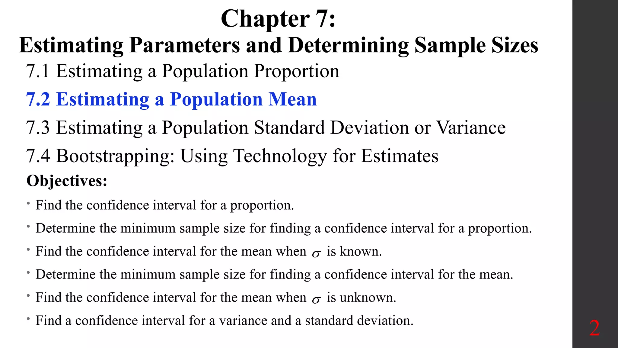
Elementary Statistics
Chapter 7: Estimating
Parameters and
Determining Sample
Sizes
7.2 Estimating a
Population Mean
1
7.1 Estimating a Population Proportion
7.2 Estimating a Population Mean
7.3 Estimating a Population Standard Deviation or Variance
7.4 Bootstrapping: Using Technology for Estimates
2
Chapter 7:
Estimating Parameters and Determining Sample Sizes
Objectives:
• Find the confidence interval for a proportion.
• Determine the minimum sample size for finding a confidence interval for a proportion.
• Find the confidence interval for the mean when  is known.
• Determine the minimum sample size for finding a confidence interval for the mean.
• Find the confidence interval for the mean when  is unknown.
• Find a confidence interval for a variance and a standard deviation.
Confidence Interval for Estimating a Population Mean with σ Not Known: Requirements
1. The sample is a simple random sample.
2. Either or both of these conditions are satisfied: The population is normally distributed or n > 30.
µ = population mean
n = number of sample values
𝑥 = sample mean
E = margin of error
s = sample standard deviation
7.2 Estimating a Population Mean
Margin of Error
Confidence
Interval
𝑋 − 𝑡𝛼
2
𝑠
𝑛
< 𝜇 < 𝑋 + 𝑡𝛼
2
𝑠
𝑛
Degrees of Freedom: df = n − 1 is the number of degrees of freedom used when finding the critical value.
Critical value: tα/2 is the critical value separating an area of α/2 in the right tail of the student t distribution.
𝑆𝑥 =
𝑠
𝑛
→ 𝐸 = 𝑡𝛼
2
𝑠
𝑛
3
𝐶𝐼: 𝑥 ± 𝐸 →
If a population has a normal distribution, then the distribution of
𝑡 =
𝑥−𝜇
𝑠/ 𝑛
is a Student t distribution for all samples of size n. A
Student t distribution is commonly referred to as a t distribution.
In general, the number of degrees of freedom for a collection of
sample data is the number of sample values that can vary after
certain restrictions have been imposed on all data values. Degrees
of freedom: df = n − 1 (if need be use the closest value in the
table or to be conservative use the next lower number of df.)
7.2 Estimating a Population Mean, Student t Distribution
The t distribution is similar to SND:
1. It is bell-shaped.
2. It is symmetric about the mean.
3. The mean, median, and mode are
equal to 0 and are located at the
center of the distribution.
4. The curve never touches the x axis. 4
The t distribution differs from SND:
1. The variance is greater than 1.
2. The t distribution is actually a family
of curves based on the concept of
degrees of freedom, which is related
to sample size.
3. As the sample size increases, the t
distribution approaches the standard
normal distribution.
Find the Critical Value
tα/2 corresponding to
95% CI, n =15
5
Example 1
Solution
n = 15,df = n − 1 = 14.
95% CL: 𝛼 = 0.05 → Area of
0.025 in each of the two tails of
the t distribution
TI Calculator:
T- Distribution: find the t-score
1. 2nd + VARS
2. invT(
3. 2 entries (Left Area,df)
4. Enter
Does garlic lowers cholesterol levels? To test the effectiveness of garlic, 49 subjects were treated with
doses of raw garlic, and their cholesterol levels were measured before and after the treatment. The
changes in their levels of LDL cholesterol (in mg/dL) have a mean of 0.4 and a standard deviation of
21.0. Use the sample statistics of n = 49, 𝑥 = 0.4, and s = 21.0 to construct a 95% confidence interval
estimate of the mean net change in LDL cholesterol after the garlic treatment. What does the
confidence interval suggest about the effectiveness of garlic in reducing LDL cholesterol?
Example 2
Given: Given: simple random sample and n = 49 (i.e., n > 30).
n = 49, 𝑥 = 0.4, and s = 21.0 , 95% CI = ?
6
𝑥 ± 𝐸, 𝑥 − 𝐸 < 𝜇 < 𝑥 + 𝐸
We are 95% confident that the limits of –5.6 and 6.4 actually do contain the
value of μ, the mean of the changes in LDL cholesterol for the population.
𝐸 = 2.009
21
49
n = 49 ⇾ df = 49 – 1 = 48,
Closest df = 50, two tails: 𝑡𝛼/2 = 2.009
= 6.027
0.4 − 6.027 < 𝜇 < 0.4 + 6.027 −5.627 < 𝜇 < 6.427
The confidence interval limits contain the value of 0, so it
is possible that the mean of the changes in LDL cholesterol
is equal to 0. This suggests that the garlic treatment did not
affect the LDL cholesterol levels. It does not appear that the
garlic treatment is effective in lowering LDL cholesterol.
𝐸 = 𝑡𝛼
2
𝑠
𝑛
TI Calculator:
Confidence Interval: T- interval
1. Stat
2. Tests
3. T - Interval
4. Enter Data (Freq:1) or Stats
(𝒙 , s & CL)
5. Enter (Calculate)
Ten randomly selected people were asked how long they slept at night.
The mean time was 7.1 hours, and the standard deviation was 0.78 hour.
Find the 95% confidence interval of the mean time. Assume the variable is
normally distributed.
Example 3
Given: ND, n = 10, 𝑥 = 7.1 hrs, and s = 0.78 hrs , 95% CI = ?
7
n = 10 ⇾ df = 10 – 1 = 9 ⇾ 𝑡𝛼/2 = 2.262
𝑋 − 𝑡𝛼
2
𝑠
𝑛
< 𝜇 < 𝑋 + 𝑡𝛼
2
𝑠
𝑛
7.1 − 2.262
0.78
10
< 𝜇 < 7.1 + 2.262
0.78
10
7.1 − 0.56 < 𝜇 < 7.1 + 0.56 6.54 < 𝜇 < 7.66
𝑥 ± 𝐸, 𝑥 − 𝐸 < 𝜇 < 𝑥 + 𝐸 𝐸 = 𝑡𝛼
2
𝑠
𝑛
TI Calculator:
Confidence Interval: T- interval
1. Stat
2. Tests
3. T - Interval
4. Enter Data (Freq:1) or Stats
(𝒙 , s & CL)
5. Enter (Calculate)
Finding the Point Estimate and E from a Confidence Interval
Point estimate of µ: 𝑥 =
𝑈𝐶𝐿+𝐿𝐶𝐿
2
, UCL: Upper Confidence Limit
Margin of error: 𝐸 =
𝑈𝐶𝐿−𝐿𝐶𝐿
2
,LCL: Lower Confidence Limit
8
7.2 Estimating a Population Mean
Determine the sample size n required to estimate the value of a population
mean µ.
Confidence Interval for Estimating a Population Mean with σ Known
𝑛 =
𝑧𝛼
2
⋅ 𝜎
𝐸
2
𝐶𝐼: 𝑥 ± 𝐸 → 𝑥 − 𝑍𝛼
2
𝜎
𝑛
< 𝜇 < 𝑥 + 𝑍𝛼
2
𝜎
𝑛
𝜎𝑥 =
𝜎
𝑛
→ 𝐸 = 𝑍𝛼
2
𝜎
𝑛
People have died in boat and aircraft accidents because an obsolete estimate of the mean weight of
men was used. The mean weight of men has increased considerably, so we need to update our estimate
of that mean so that boats, aircraft, elevators, etc. do not become dangerously overloaded. Using the
weights of men from a random sample, we obtain these sample statistics for the simple random sample:
n = 40 and 𝑥 = 172.55 lb. Research from several other sources suggests that the population of weights
of men has a standard deviation given by σ = 26 lb.
Example 4
Given: Random sample and n = 40 ( n > 30), n = 40, 𝑥 = 172.55lb, and σ = 26 lb, 95% CI = ?
9
𝐸 = 1.96
26
40
α = 0.05, so zα/2= ± 1.96
= 8.0575
172.55 − 8.0575 < 𝜇 < 172.55 − 8.0575
PE of 𝝁 = 𝒙 = 172.55lb
164.49 < 𝜇 < 180.61
a. Find the point estimate (PE) of the mean weight of the population of all men.
b. Construct a 95% confidence interval estimate of the mean weight of all men.
Based on the confidence interval, it is possible that the mean weight of 166.3 lb
used in 1960 could be the mean weight of men today. However, the best point
estimate of 172.55 lb suggests that the mean weight of men is now considerably
greater than 166.3 lb. An underestimate of the mean weight of men could result
in lives lost through overloaded boats and aircraft, these results strongly suggest
that additional data should be collected.
𝑥 ± 𝐸, 𝑥 − 𝐸 < 𝜇 < 𝑥 + 𝐸
c. What do the results suggest about the mean weight of 166.3 lb
that was used to determine the safe TI Calculator:
Confidence Interval:
Z - interval
1. Stat
2. Tests
3. Z - Interval
4. Enter Data or Stats
(𝒙 , σ & CL)
𝐸 = 𝑡𝛼
2
𝑠
𝑛
, 𝐸 = 𝑍𝛼
2
𝜎
𝑛
A researcher wishes to estimate the number of days it takes a car dealer to sell a particular brand of car. A
sample of 50 such cars had a mean time on the dealer’s lot of 54 days. Assume the population standard
deviation to be 6.0 days. Find the best point estimate of the population mean and the 95% confidence
interval of the population mean.
Example 5
Given: Random sample and n = 50 (n > 30)
n = 50, 𝑥 = 54, and σ = 6, 95% CI = ?
10
𝑋 = 54, 𝜎 = 6.0, 𝑛 = 50,95% → 𝑧 = 1.96
PE of 𝜇 = 𝑥 = 54
54 − 1.96
6.0
50
< 𝜇 < 54 + 1.96
6.0
50
54 − 1.7 < 𝜇 < 54 + 1.7
52.3 < 𝜇 < 55.7
52 < 𝜇 < 56
𝑥 ± 𝐸, 𝑥 − 𝐸 < 𝜇 < 𝑥 + 𝐸 𝐸 = 𝑡𝛼
2
𝑠
𝑛
, 𝐸 = 𝑍𝛼
2
𝜎
𝑛
A survey of 30 emergency room patients found that the average waiting time for
treatment was 174.3 minutes. Assuming that the population standard deviation is 46.5
minutes, find the best point estimate of the population mean and the 99% confidence of
the population mean.
Example 6
Given: Random sample and n = 30 , 𝑥 = 174.3 min,
and σ = 46.5 min, 99% CI = ?
11
99% → 𝑧 = 2.575
PE of 𝜇 = 𝑥 = 174.3min
174.3 − 2.575
46.5
30
< 𝜇 < 174.3 + 2.575
46.5
30
174.3 − 21.861 < 𝜇 < 174.3 + 21.861 152.439 < 𝜇 < 196.161
0.005
0.005
𝑥 ± 𝐸, 𝑥 − 𝐸 < 𝜇 < 𝑥 + 𝐸 𝐸 = 𝑡𝛼
2
𝑠
𝑛
, 𝐸 = 𝑍𝛼
2
𝜎
𝑛
How many statistics students must be randomly selected for IQ
tests if we want 95% confidence that the sample mean is within 3 IQ points of
the population mean? Assume normal distribution with σ =15
12
Example 7
=
1.96 ⋅ 15
3
2
= 96.04 → 𝑛 = 97
Example 8: A scientist wishes to estimate the average depth of a river. He wants to
be 99% confident that the estimate is accurate within 2 feet. From a previous study, the
standard deviation of the depths measured was 4.33 feet. How large a sample is
required?
99% → 𝑧 = 2.575, 𝐸 = 2, 𝜎 = 4.33
=
2.575 • 4.33
2
2
95% → 𝑧 = 1.96
𝐸 = 3, 𝜎 = 15
𝑛 =
𝑧𝛼
2
⋅ 𝜎
𝐸
2
𝑛 =
𝑧𝛼
2
⋅ 𝜎
𝐸
2
𝑛 =
𝑧𝛼
2
⋅ 𝜎
𝐸
2
= 31.07 → 𝑛 = 32
13
Example 9 (Time)
Solution: Requirement Check:
(1) The sample is a simple random sample.
(2) n = 15 < 30, so we need to investigate normality.
Sample data appear to
be from a normally
distributed population.
𝐶𝐼: 𝑥 ± 𝐸 →
30.9 ± 1.4760
29.4ℎ𝑔 < 𝜇 < 32.4ℎ𝑔
𝐸 = 1.96
2.9
15
= 1.4760
Given the following Random sample data for n = 15
, 𝑥 = 30.9 hg, and σ = 2.9 hg for birth weights of
girls, construct a 959% CI of the mean birth
weight of all girls.
33 28 33 37 31 32 31 28
34 28 33 26 30 31 28
𝑥 ± 𝐸, 𝑥 − 𝐸 < 𝜇 < 𝑥 + 𝐸 𝐸 = 𝑡𝛼
2
𝑠
𝑛
, 𝐸 = 𝑍𝛼
2
𝜎
𝑛
Choosing an Appropriate Distribution: t or Z
Conditions Method
σ not known and normally distributed population
or σ not known and n > 30
Use student t distribution
σ known and normally distributed population or σ
known and n > 30 (In reality, σ is rarely known.)
Use normal (z) distribution.
Population is not normally distributed and n ≤ 30. Use the bootstrapping method
or a nonparametric method.
14
Dealing with Unknown σ When Finding Sample Size
1. Use the range rule of thumb to estimate the standard deviation as follows: σ
 range/4, where the range is determined from sample data.
2. Start the sample collection process without knowing σ and, using the first
several values, calculate the sample standard deviation s and use it in place
of σ. The estimated value of σ can then be improved as more sample data
are obtained, and the sample size can be refined accordingly.
3. Estimate the value of σ by using the results of some other earlier study.
15
Dealing with Unknown σ When Finding Critical values
a. Find the critical t value for α = 0.05 with df = 16 for a right-tailed t test.
Find the 0.05 column in the top row and 16 in the left-hand column.
The critical t value is +1.746.
16
b. Find the critical t value for α = 0.01 with d.f. = 22 for
a left-tailed test.
Find the 0.01 column in the One tail
row, and 22 in the d.f. column.
The critical value is t = –2.508 since
the test is a one-tailed left test.
c. Find the critical value for α = 0.10 with d.f. = 18 for a
two-tailed t test.
Find the 0.10 column in the Two tails row, and 18 in the d.f.
column. The critical values are 1.734 and –1.734.

Estimating a Population Mean

  • 1.
    Elementary Statistics Chapter 7:Estimating Parameters and Determining Sample Sizes 7.2 Estimating a Population Mean 1
  • 2.
    7.1 Estimating aPopulation Proportion 7.2 Estimating a Population Mean 7.3 Estimating a Population Standard Deviation or Variance 7.4 Bootstrapping: Using Technology for Estimates 2 Chapter 7: Estimating Parameters and Determining Sample Sizes Objectives: • Find the confidence interval for a proportion. • Determine the minimum sample size for finding a confidence interval for a proportion. • Find the confidence interval for the mean when  is known. • Determine the minimum sample size for finding a confidence interval for the mean. • Find the confidence interval for the mean when  is unknown. • Find a confidence interval for a variance and a standard deviation.
  • 3.
    Confidence Interval forEstimating a Population Mean with σ Not Known: Requirements 1. The sample is a simple random sample. 2. Either or both of these conditions are satisfied: The population is normally distributed or n > 30. µ = population mean n = number of sample values 𝑥 = sample mean E = margin of error s = sample standard deviation 7.2 Estimating a Population Mean Margin of Error Confidence Interval 𝑋 − 𝑡𝛼 2 𝑠 𝑛 < 𝜇 < 𝑋 + 𝑡𝛼 2 𝑠 𝑛 Degrees of Freedom: df = n − 1 is the number of degrees of freedom used when finding the critical value. Critical value: tα/2 is the critical value separating an area of α/2 in the right tail of the student t distribution. 𝑆𝑥 = 𝑠 𝑛 → 𝐸 = 𝑡𝛼 2 𝑠 𝑛 3 𝐶𝐼: 𝑥 ± 𝐸 →
  • 4.
    If a populationhas a normal distribution, then the distribution of 𝑡 = 𝑥−𝜇 𝑠/ 𝑛 is a Student t distribution for all samples of size n. A Student t distribution is commonly referred to as a t distribution. In general, the number of degrees of freedom for a collection of sample data is the number of sample values that can vary after certain restrictions have been imposed on all data values. Degrees of freedom: df = n − 1 (if need be use the closest value in the table or to be conservative use the next lower number of df.) 7.2 Estimating a Population Mean, Student t Distribution The t distribution is similar to SND: 1. It is bell-shaped. 2. It is symmetric about the mean. 3. The mean, median, and mode are equal to 0 and are located at the center of the distribution. 4. The curve never touches the x axis. 4 The t distribution differs from SND: 1. The variance is greater than 1. 2. The t distribution is actually a family of curves based on the concept of degrees of freedom, which is related to sample size. 3. As the sample size increases, the t distribution approaches the standard normal distribution.
  • 5.
    Find the CriticalValue tα/2 corresponding to 95% CI, n =15 5 Example 1 Solution n = 15,df = n − 1 = 14. 95% CL: 𝛼 = 0.05 → Area of 0.025 in each of the two tails of the t distribution TI Calculator: T- Distribution: find the t-score 1. 2nd + VARS 2. invT( 3. 2 entries (Left Area,df) 4. Enter
  • 6.
    Does garlic lowerscholesterol levels? To test the effectiveness of garlic, 49 subjects were treated with doses of raw garlic, and their cholesterol levels were measured before and after the treatment. The changes in their levels of LDL cholesterol (in mg/dL) have a mean of 0.4 and a standard deviation of 21.0. Use the sample statistics of n = 49, 𝑥 = 0.4, and s = 21.0 to construct a 95% confidence interval estimate of the mean net change in LDL cholesterol after the garlic treatment. What does the confidence interval suggest about the effectiveness of garlic in reducing LDL cholesterol? Example 2 Given: Given: simple random sample and n = 49 (i.e., n > 30). n = 49, 𝑥 = 0.4, and s = 21.0 , 95% CI = ? 6 𝑥 ± 𝐸, 𝑥 − 𝐸 < 𝜇 < 𝑥 + 𝐸 We are 95% confident that the limits of –5.6 and 6.4 actually do contain the value of μ, the mean of the changes in LDL cholesterol for the population. 𝐸 = 2.009 21 49 n = 49 ⇾ df = 49 – 1 = 48, Closest df = 50, two tails: 𝑡𝛼/2 = 2.009 = 6.027 0.4 − 6.027 < 𝜇 < 0.4 + 6.027 −5.627 < 𝜇 < 6.427 The confidence interval limits contain the value of 0, so it is possible that the mean of the changes in LDL cholesterol is equal to 0. This suggests that the garlic treatment did not affect the LDL cholesterol levels. It does not appear that the garlic treatment is effective in lowering LDL cholesterol. 𝐸 = 𝑡𝛼 2 𝑠 𝑛 TI Calculator: Confidence Interval: T- interval 1. Stat 2. Tests 3. T - Interval 4. Enter Data (Freq:1) or Stats (𝒙 , s & CL) 5. Enter (Calculate)
  • 7.
    Ten randomly selectedpeople were asked how long they slept at night. The mean time was 7.1 hours, and the standard deviation was 0.78 hour. Find the 95% confidence interval of the mean time. Assume the variable is normally distributed. Example 3 Given: ND, n = 10, 𝑥 = 7.1 hrs, and s = 0.78 hrs , 95% CI = ? 7 n = 10 ⇾ df = 10 – 1 = 9 ⇾ 𝑡𝛼/2 = 2.262 𝑋 − 𝑡𝛼 2 𝑠 𝑛 < 𝜇 < 𝑋 + 𝑡𝛼 2 𝑠 𝑛 7.1 − 2.262 0.78 10 < 𝜇 < 7.1 + 2.262 0.78 10 7.1 − 0.56 < 𝜇 < 7.1 + 0.56 6.54 < 𝜇 < 7.66 𝑥 ± 𝐸, 𝑥 − 𝐸 < 𝜇 < 𝑥 + 𝐸 𝐸 = 𝑡𝛼 2 𝑠 𝑛 TI Calculator: Confidence Interval: T- interval 1. Stat 2. Tests 3. T - Interval 4. Enter Data (Freq:1) or Stats (𝒙 , s & CL) 5. Enter (Calculate)
  • 8.
    Finding the PointEstimate and E from a Confidence Interval Point estimate of µ: 𝑥 = 𝑈𝐶𝐿+𝐿𝐶𝐿 2 , UCL: Upper Confidence Limit Margin of error: 𝐸 = 𝑈𝐶𝐿−𝐿𝐶𝐿 2 ,LCL: Lower Confidence Limit 8 7.2 Estimating a Population Mean Determine the sample size n required to estimate the value of a population mean µ. Confidence Interval for Estimating a Population Mean with σ Known 𝑛 = 𝑧𝛼 2 ⋅ 𝜎 𝐸 2 𝐶𝐼: 𝑥 ± 𝐸 → 𝑥 − 𝑍𝛼 2 𝜎 𝑛 < 𝜇 < 𝑥 + 𝑍𝛼 2 𝜎 𝑛 𝜎𝑥 = 𝜎 𝑛 → 𝐸 = 𝑍𝛼 2 𝜎 𝑛
  • 9.
    People have diedin boat and aircraft accidents because an obsolete estimate of the mean weight of men was used. The mean weight of men has increased considerably, so we need to update our estimate of that mean so that boats, aircraft, elevators, etc. do not become dangerously overloaded. Using the weights of men from a random sample, we obtain these sample statistics for the simple random sample: n = 40 and 𝑥 = 172.55 lb. Research from several other sources suggests that the population of weights of men has a standard deviation given by σ = 26 lb. Example 4 Given: Random sample and n = 40 ( n > 30), n = 40, 𝑥 = 172.55lb, and σ = 26 lb, 95% CI = ? 9 𝐸 = 1.96 26 40 α = 0.05, so zα/2= ± 1.96 = 8.0575 172.55 − 8.0575 < 𝜇 < 172.55 − 8.0575 PE of 𝝁 = 𝒙 = 172.55lb 164.49 < 𝜇 < 180.61 a. Find the point estimate (PE) of the mean weight of the population of all men. b. Construct a 95% confidence interval estimate of the mean weight of all men. Based on the confidence interval, it is possible that the mean weight of 166.3 lb used in 1960 could be the mean weight of men today. However, the best point estimate of 172.55 lb suggests that the mean weight of men is now considerably greater than 166.3 lb. An underestimate of the mean weight of men could result in lives lost through overloaded boats and aircraft, these results strongly suggest that additional data should be collected. 𝑥 ± 𝐸, 𝑥 − 𝐸 < 𝜇 < 𝑥 + 𝐸 c. What do the results suggest about the mean weight of 166.3 lb that was used to determine the safe TI Calculator: Confidence Interval: Z - interval 1. Stat 2. Tests 3. Z - Interval 4. Enter Data or Stats (𝒙 , σ & CL) 𝐸 = 𝑡𝛼 2 𝑠 𝑛 , 𝐸 = 𝑍𝛼 2 𝜎 𝑛
  • 10.
    A researcher wishesto estimate the number of days it takes a car dealer to sell a particular brand of car. A sample of 50 such cars had a mean time on the dealer’s lot of 54 days. Assume the population standard deviation to be 6.0 days. Find the best point estimate of the population mean and the 95% confidence interval of the population mean. Example 5 Given: Random sample and n = 50 (n > 30) n = 50, 𝑥 = 54, and σ = 6, 95% CI = ? 10 𝑋 = 54, 𝜎 = 6.0, 𝑛 = 50,95% → 𝑧 = 1.96 PE of 𝜇 = 𝑥 = 54 54 − 1.96 6.0 50 < 𝜇 < 54 + 1.96 6.0 50 54 − 1.7 < 𝜇 < 54 + 1.7 52.3 < 𝜇 < 55.7 52 < 𝜇 < 56 𝑥 ± 𝐸, 𝑥 − 𝐸 < 𝜇 < 𝑥 + 𝐸 𝐸 = 𝑡𝛼 2 𝑠 𝑛 , 𝐸 = 𝑍𝛼 2 𝜎 𝑛
  • 11.
    A survey of30 emergency room patients found that the average waiting time for treatment was 174.3 minutes. Assuming that the population standard deviation is 46.5 minutes, find the best point estimate of the population mean and the 99% confidence of the population mean. Example 6 Given: Random sample and n = 30 , 𝑥 = 174.3 min, and σ = 46.5 min, 99% CI = ? 11 99% → 𝑧 = 2.575 PE of 𝜇 = 𝑥 = 174.3min 174.3 − 2.575 46.5 30 < 𝜇 < 174.3 + 2.575 46.5 30 174.3 − 21.861 < 𝜇 < 174.3 + 21.861 152.439 < 𝜇 < 196.161 0.005 0.005 𝑥 ± 𝐸, 𝑥 − 𝐸 < 𝜇 < 𝑥 + 𝐸 𝐸 = 𝑡𝛼 2 𝑠 𝑛 , 𝐸 = 𝑍𝛼 2 𝜎 𝑛
  • 12.
    How many statisticsstudents must be randomly selected for IQ tests if we want 95% confidence that the sample mean is within 3 IQ points of the population mean? Assume normal distribution with σ =15 12 Example 7 = 1.96 ⋅ 15 3 2 = 96.04 → 𝑛 = 97 Example 8: A scientist wishes to estimate the average depth of a river. He wants to be 99% confident that the estimate is accurate within 2 feet. From a previous study, the standard deviation of the depths measured was 4.33 feet. How large a sample is required? 99% → 𝑧 = 2.575, 𝐸 = 2, 𝜎 = 4.33 = 2.575 • 4.33 2 2 95% → 𝑧 = 1.96 𝐸 = 3, 𝜎 = 15 𝑛 = 𝑧𝛼 2 ⋅ 𝜎 𝐸 2 𝑛 = 𝑧𝛼 2 ⋅ 𝜎 𝐸 2 𝑛 = 𝑧𝛼 2 ⋅ 𝜎 𝐸 2 = 31.07 → 𝑛 = 32
  • 13.
    13 Example 9 (Time) Solution:Requirement Check: (1) The sample is a simple random sample. (2) n = 15 < 30, so we need to investigate normality. Sample data appear to be from a normally distributed population. 𝐶𝐼: 𝑥 ± 𝐸 → 30.9 ± 1.4760 29.4ℎ𝑔 < 𝜇 < 32.4ℎ𝑔 𝐸 = 1.96 2.9 15 = 1.4760 Given the following Random sample data for n = 15 , 𝑥 = 30.9 hg, and σ = 2.9 hg for birth weights of girls, construct a 959% CI of the mean birth weight of all girls. 33 28 33 37 31 32 31 28 34 28 33 26 30 31 28 𝑥 ± 𝐸, 𝑥 − 𝐸 < 𝜇 < 𝑥 + 𝐸 𝐸 = 𝑡𝛼 2 𝑠 𝑛 , 𝐸 = 𝑍𝛼 2 𝜎 𝑛
  • 14.
    Choosing an AppropriateDistribution: t or Z Conditions Method σ not known and normally distributed population or σ not known and n > 30 Use student t distribution σ known and normally distributed population or σ known and n > 30 (In reality, σ is rarely known.) Use normal (z) distribution. Population is not normally distributed and n ≤ 30. Use the bootstrapping method or a nonparametric method. 14
  • 15.
    Dealing with Unknownσ When Finding Sample Size 1. Use the range rule of thumb to estimate the standard deviation as follows: σ  range/4, where the range is determined from sample data. 2. Start the sample collection process without knowing σ and, using the first several values, calculate the sample standard deviation s and use it in place of σ. The estimated value of σ can then be improved as more sample data are obtained, and the sample size can be refined accordingly. 3. Estimate the value of σ by using the results of some other earlier study. 15
  • 16.
    Dealing with Unknownσ When Finding Critical values a. Find the critical t value for α = 0.05 with df = 16 for a right-tailed t test. Find the 0.05 column in the top row and 16 in the left-hand column. The critical t value is +1.746. 16 b. Find the critical t value for α = 0.01 with d.f. = 22 for a left-tailed test. Find the 0.01 column in the One tail row, and 22 in the d.f. column. The critical value is t = –2.508 since the test is a one-tailed left test. c. Find the critical value for α = 0.10 with d.f. = 18 for a two-tailed t test. Find the 0.10 column in the Two tails row, and 18 in the d.f. column. The critical values are 1.734 and –1.734.