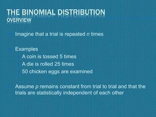
The document provides an overview of the binomial distribution including its basics, prerequisites, and examples. It defines a binomial experiment as having a fixed number of independent trials where each trial results in one of two possible outcomes (success or failure) with a constant probability. The document gives examples of flipping a coin and throwing a die to illustrate binomial experiments. It also provides notation used in binomial distributions and shows how to determine if an experiment follows a binomial distribution.

1. THE BINOMIAL
DISTRIBUTION
& ITS
APPLICATIONS
Presented By: Umar Farooq, Umair Javed, Shamim Aslam, Hamza Akash
& ,Haseeb Hayat

2. BINOMIAL DISTRIBUTION
The main objective of this is to cover the basics of binomial distribution,
study some examples and look at its Advantages and Disadvantages.

3. BASICS
Before we begin new content, we should review a few terms from previous lessons that
we will see again in
this lesson:
 Discrete: Data that can only take on set number of values
 Continuous: Quantitative data that can take on any value between the minimum and
maximum, and any value between two other values
 Probability: The likelihood of an event occuring ; P(A)=number of events considered
outcome A number of total eventsP(A) = number of events considered out come A
number of total events
 P(A∩B)P(A∩B): Intersection of A and B; "probability of A and B"
 P(A∪B)P(A∪B): Union of A and B; "probability of A or B" (this also includes the
probability of A and B)
 Mean: The numerical average calculated as the sum of all of the data values divided
by the number of values; represented as X¯¯¯¯X¯.
 Standard deviation: Roughly the average difference between individual data and
the mean; for a sample, represented as s, s=∑(x−x¯¯¯)2n−1−−−−−−√s=∑(x−x¯)2n−1
 Sample: A subset of the population from which data is actually collected
 Population: The entire set of possible observations in which we are interested
 Statistic: A measure concerning a sample (e.g., sample mean)
 Parameter: A measure concerning a population (e.g., population mean)

4. PROBABILITY DISTRIBUTION PREREQUISITES
To understand probability distributions, it is
important to understand variables. Random
variables, and some notation.
 A variable is a symbol (A, B, x, y, etc.) that can take on any
of a specified set of values.
 When the value of a variable is the outcome of a statistical
experiment, that variable is a random variable.
Generally, statisticians use a capital letter to represent a
random
variable and
a lower-case letter, to represent one of its values. For example,
 X represents the random variable X.
 P(X) represents the probability of X.
 P(X = x) refers to the probability that the random variable X is
equal to a particular value, denoted by x. As an example, P(X
= 1) refers to the probability that the random variable X is

5. RANDOM VARIABLE
The mathematical rule (or function) that assigns a
given numerical value to each possible
outcome of an experiment in the sample space
of interest.
 Discrete random variables
 Continuous random variables

6. WHAT ARE PROBABILITY DISTRIBUTIONS?
A probability distribution is a table or an equation that
links each outcome of a statistical experiment with
its probability of occurrence.
 A discrete probability distribution specifies:
the possible values of the random variable, and
the probability that each outcome will occur

7. PROBABILTY DISTRIBUTIONS
An example will make clear the relationship between random
variables and probability distributions. Suppose you flip a coin two
times. This simple statistical experiment can have four possible
outcomes: HH, HT, TH, and TT. Now, let the variable X represent
the number of Heads that result from this experiment. The
variable X can take on the values 0, 1, or 2. In this example, X is
a random variable; because its value is determined by the
outcome of a statistical experiment.
A probability distribution is a table or an equation that links each
outcome of a statistical experiment with its probability of
occurrence. Consider the coin flip experiment described above.
The table below, which associates each outcome with its
probability, is an example of a probability distribution.
Number of Heads Probability
0 0.25
1 0.50
2 0.25
Distribution Table

8. DISTRIBUTIONS
Here are some of the common distributions and some of the reasons that they are
useful:
 Normal: This is useful for looking at means and other linear combinations (e.g.
regression coefficients) because of the CLT. Related to that is if something is known
to arise due to additive effects of many different small causes then the normal may
be a reasonable distribution: for example, many biological measures are the result of
multiple genes and multiple environmental factors and therefor are often
approximately normal.
 Gamma: Right skewed and useful for things with a natural minimum at 0. Commonly
used for elapsed times and some financial variables.
 Exponential: special case of the Gamma. It is memoryless and scales easily.
 Chi-squared (χ2χ2): special case of the Gamma. Arises as sum of squared normal
variables (so used for variances).
 Beta: Defined between 0 and 1 (but could be transformed to be between other
values), useful for proportions or other quantities that must be between 0 and 1.
 Binomial: How many "successes" out of a given number of independent trials with
same probability of "success".
 Poisson: Common for counts. Nice properties that if the number of events in a period
of time or area follows a Poisson, then the number in twice the time or area still
follows the Poisson (with twice the mean): this works for adding Poissons or scaling
with values other than 2.
You could use a tree diagram

9. GRAPHS OF SOME DISTRIBUTIONS

10. PROBABILITY DISTRIBUTIONS
 We use probability
distributions because
they work –they fit lots
of data in real world

11. TRY THIS
Have you got a coin?
Toss it six times in a roll, each time counting
the number of times the result, ‘heads’ is
observed.

12. BINOMIAL EXPERIMENT
 There are many probability experiments for
which the results of each trial can be reduced
to two outcomes: success and failure.
 For instance, when a basketball player
attempts a free throw, he or she either makes
the basket or does not. Probability
experiments such as these are called
binomial experiments.

13. OBSERVED PROBABILITY
Before a coin is tossed six times in a roll,
what is the probability that in total there will
be two ‘heads’ out of six?

14. BERNOULLI TRIAL
Tossing a coin is Bernoulli trial. A Bernoulli trial is a
random experiment that has only two, mutually
exclusive outcomes.
Thus, when a coin is tossed, the two possible
outcomes are revealing a ‘heads’ or revealing a
‘tails’. We want to see how many ‘heads’ are
revealed. So revealing a ‘heads’ is a ‘success’.
Revealing a ‘tails’ is a ‘failure’.

15. PROPERTIES OF A BERNOULLI TRIAL
Since you’re tossing the same coin in all six
Bernoulli trials, the probability of a ‘heads’ or
a
success, p, is the same for each repeat of
the
Bernoulli trial
But the coin has no memory: Bernoulli trials are
independent

16. MULTIPLE ANSWER QUESTION: WHICH OF THE
FOLLOWING ARE REPEATS OF BERNOULLI
TRIALS
1.The game of joker’s challenge is played with
the full deck of cards: The player is shown a card,
and s/he calls whether the next card will be lower
or higher, if the call is correct the game is
repeated, and so on
2.A box contains 20 packs of chocolate, 8 of
which are milk. Selecting a chocolate, checking if
its milk, eating eat it, really enjoying it and then
repeating the exercise.

17. BINOMIAL DISTRIBUTION
"Bi" means "two" (like a bicycle has two
wheels) ...
... so this is about things with two results.

18. FLIPPING A COIN
Tossing a Coin:
Did we get Heads (H)
or
Tails (T)
We say the probability of the coin landing H is ½
And the probability of the coin landing T is ½

19. THROWING A DIE
Throwing a Die:
 Did we get a four ... ?
 ... or not?
 We say the probability of a four is 1/6 (one of
the six faces is a four).
And the probability of not four is 5/6 (five of
the six faces are not a four)

20. DEFINATION
 A binomial experiment is a probability experiment that
satisfies the following conditions:
1. The experiment is repeated for a fixed number of
trials, where each trial is independent of the other
trials.
2. There are only two possible outcomes of interest for
each trial. The outcomes can be classified as a
success (S) or as a failure (F).
3. The probability of a success, P(S), is the same for
each trial.
4. The random variable, x, counts the number of
successful trials

21. NOTATION FOR BINOMIAL EXPERIMENTS
Symbol Description
n The number of times a trial is repeated.
p = P(S) The probability of success in a single
trial.
q = P(F) The probability of failure in a single trial
(q = 1 – p)
x The random variable represents a
count of the number of successes in n
trials: x = 0, 1, 2, 3, . . . n.

22. HOW TO DETERMINE?
 Decide whether the experiment is a binomial
experiment. If it is, specify the values of n, p
and q and list the possible values of the
random variable, x. If it is not, explain why.
A certain surgical procedure has an 85%
chance of success. A doctor performs the
procedure on eight patients. The random
variable represents the number of successful
surgeries.

23. BINOMIAL EXPERIMENTS
Solution: the experiment is a binomial experiment
because it satisfies the four conditions of a
binomial experiment. In the experiment, each
surgery represents one trial. There are eight
surgeries, and each surgery is independent of
the others. Also, there are only two possible
outcomes for each surgery—either the surgery
is a success or it is a failure. Finally, the
probability of success for each surgery is 0.85.
n = 8
p = 0.85
q = 1 – 0.85 = 0.15
x = 0, 1, 2, 3, 4, 5, 6, 7, 8

24. BINOMIAL EXPERIMENTS
2. A jar contains five red marbles, nine blue
marbles and six green marbles. You
randomly select three marbles from the jar,
without replacement. The random variable
represents the number of red marbles.

25. BINOMIAL EXPERIMENTS
Solution: The experiment is not a binomial
experiment because it does not satisfy all four
conditions of a binomial experiment. In the
experiment, each marble selection represents
one trial and selecting a red marble is a
success. When selecting the first marble, the
probability of success is 5/20. However
because the marble is not replaced, the
probability is no longer 5/20. So the trials are
not independent, and the probability of a
success is not the same for each trial.

26. BINOMIAL EXAMPLE
Take the example of 5 coin tosses. What’s
the probability that you flip exactly 3 heads
in 5 coin tosses?

27. LET’S TOSS A COIN
HEAD HEAD HEAD
TAIL HEAD HEAD
HEAD HEAD TAIL
HEAD TAIL HEAD
HEAD TAIL TAIL
TAIL HEAD TAIL
TAIL TAIL HEAD
TAIL TAIL TAIL
Toss a fair coin threetimes ...
what is the chance of
getting two Heads?
Tossing a coin three times
(H is for heads, T for Tails)
Can get any of these
8 outcomes:

28. Which outcomes do we want?
"Two Heads" could be in any order: "HHT", "THH" and
"HTH" all
have two Heads (and one Tail).
 So 3 of the outcomes produce "Two Heads".
What is the probability of each outcome?
 Each outcome is equally likely, and there are 8 of them.
So each has a probability of 1/8
So the probability of event "Two Heads" is:
Number of outcomes we want * Probability of each
outcome
3 × 1/8 = 3/8

29. LETS CALCULATE THEM ALL
The calculations are (P means "Probability of"):
 P(Three Heads) = P(HHH) = 1/8
 P(Two Heads) = P(HHT) + P(HTH) + P(THH) = 1/8 + 1/8 + 1/8
= 3/8
 P(One Head) = P(HTT) + P(THT) + P(TTH) = 1/8 + 1/8 + 1/8
= 3/8
 P(Zero Heads) = P(TTT) = 1/8
We can write this in terms of a Random Variable, X, = "The number
of
Heads from 3 tosses of a coin":
 P(X = 3) = 1/8
 P(X = 2) = 3/8
 P(X = 1) = 3/8
 P(X = 0) = 1/8

30. THE BINOMIAL DISTRIBUTION
BERNOULLI RANDOM VARIABLES
 Imagine a simple trial with only two possible outcomes
 Success (S)
 Failure (F)
 Examples
 Toss of a coin (heads or tails)
 Sex of a newborn (male or female)
 Survival of an organism in a region (live or die)
Jacob Bernoulli (1654-1705)

31. THE BINOMIAL DISTRIBUTION
OVERVIEW
 Suppose that the probability of success is p
 What is the probability of failure?
 q = 1 – p
 Examples
 Toss of a coin (S = head): p = 0.5  q = 0.5
 Roll of a die (S = 1): p = 0.1667  q = 0.8333
 Fertility of a chicken egg (S = fertile): p = 0.8  q =
0.2

32. THE BINOMIAL DISTRIBUTION
OVERVIEW
 Imagine that a trial is repeated n times
 Examples
 A coin is tossed 5 times
 A die is rolled 25 times
 50 chicken eggs are examined
 Assume p remains constant from trial to trial and that the
trials are statistically independent of each other

33. THE BINOMIAL DISTRIBUTION
OVERVIEW
 What is the probability of obtaining x successes in n
trials?
 Example
 What is the probability of obtaining 2 heads from a
coin that was tossed 5 times?
P(HHTTT) = (1/2)5 = 1/32

34. THE BINOMIAL DISTRIBUTION
OVERVIEW
 But there are more possibilities:
HHTTT HTHTT HTTHT HTTTH
THHTT THTHT THTTH
TTHHT TTHTH
TTTHH
P(2 heads) = 10 × 1/32 = 10/32

35. THE BINOMIAL DISTRIBUTION
OVERVIEW
 In general, if trials result in a series of success and
failures,
FFSFFFFSFSFSSFFFFFSF…
Then the probability of x successes in that order is
P(x)= q  q  p  q  
= px  qn – x

36. THE BINOMIAL DISTRIBUTION
OVERVIEW
 However, if order is not important, then
where is the number of ways to obtain x
successes
in n trials, and i! = i  (i – 1)  (i – 2)  …  2  1
n!
x!(n – x)!
px  qn – xP(x) =
n!
x!(n – x)!

37. EXAMPLE
As voters exit the polls, you ask a representative random
sample of 6 voters if they voted for proposition 100. If
the true percentage of voters who vote for the
proposition is 55.1%, what is the probability that, in your
sample, exactly 2 voted for the proposition and 4 did
not?

38. SOLUTION:
Outcome Probability
YYNNNN = (.551)2 x (.449)4
NYYNNN (.449)1 x (.551)2 x (.449)3 = (.551)2 x (.449)4
NNYYNN (.449)2 x (.551)2 x (.449)2 = (.551)2 x (.449)4
NNNYYN (.449)3 x (.551)2 x (.449)1 = (.551)2 x (.449)4
NNNNYY (.449)4 x (.551)2 = (.551)2 x (.449)4
.
.
ways to
arrange 2
Obama votes
among 6
voters





 6
2
15 arrangements x (.551)2 x (.449)4





 6
2
P(2 yes votes exactly) = x (.551)2 x (.449)4 = 18.5%

39. BINOMIAL PROBABILITIES
There are several ways to find the probability of x
successes in n trials of a binomial experiment.
One way is to use the binomial probability
formula.
Binomial Probability Formula
In a binomial experiment, the probability of exactly
x successes in n trials is:
xnxxnx
xn qp
xxn
n
qpCxP 


!)!(
!
)(

40. BINOMIAL EXAMPLE
Take the example of 5 coin tosses. What’s
the probability that you flip exactly 3 heads
in 5 coin tosses?

41. BINOMIAL DISTRIBUTION
Solution:
One way to get exactly 3 heads: HHHTT
What’s the probability of this exact arrangement?
P(heads)xP(heads) xP(heads)xP(tails)xP(tails)
=(1/2)3 x (1/2)2
Another way to get exactly 3 heads: THHHT
Probability of this exact outcome = (1/2)1 x (1/2)3 x
(1/2)1 = (1/2)3 x (1/2)2

42. BINOMIAL DISTRIBUTION
In fact, (1/2)3 x (1/2)2 is the probability of each
unique outcome that has exactly 3 heads and 2
tails.
So, the overall probability of 3 heads and 2 tails
is:
(1/2)3 x (1/2)2 + (1/2)3 x (1/2)2 + (1/2)3 x (1/2)2 +
….. for as many unique arrangements as there
are—but how many are there??

43. Outcome Probability
THHHT (1/2)3 x (1/2)2
HHHTT (1/2)3 x (1/2)2
TTHHH (1/2)3 x (1/2)2
HTTHH (1/2)3 x (1/2)2
HHTTH (1/2)3 x (1/2)2
THTHH (1/2)3 x (1/2)2
HTHTH (1/2)3 x (1/2)2
HHTHT (1/2)3 x (1/2)2
THHTH (1/2)3 x (1/2)2
HTHHT (1/2)3 x (1/2)2
10 arrangements x (1/2)3 x (1/2)2
The probability
of each unique
outcome (note:
they are all
equal)
ways to
arrange 3
heads in
5 trials





 5
3
5C3 = 5!/3!2! = 10

44. P(3 heads and 2 tails) = x P(heads)3 x P(tails)2 =
10 x (½)5=31.25%





 5
3

45. x
p(x)
0 3 4 51 2
BINOMIAL DISTRIBUTION FUNCTION:
X= THE NUMBER OF HEADS TOSSED IN 5 COIN
TOSSES
number of heads
p(x)
number of heads

46. BINOMIAL DISTRIBUTION, GENERALLY
XnX
n
X
pp 






)1(
1-p = probability
of failure
p =
probability of
success
X = #
successes
out of n
trials
n = number of trials
Note the general pattern emerging  if you have only two possible
outcomes (call them 1/0 or yes/no or success/failure) in n independent
trials, then the probability of exactly X “successes”=

47. FINDING BINOMIAL PROBABILITIES
A six sided die is rolled 3 times. Find the probability of
rolling exactly one 6.
Roll 1 Roll 2 Roll 3 Frequency # of 6’s Probability
(1)(1)(1) = 1 3 1/216
(1)(1)(5) = 5 2 5/216
(1)(5)(1) = 5 2 5/216
(1)(5)(5) = 25 1 25/216
(5)(1)(1) = 5 2 5/216
(5)(1)(5) = 25 1 25/216
(5)(5)(1) = 25 1 25/216
(5)(5)(5) = 125 0 125/216
You could use a
tree diagram

48. FINDING BINOMIAL PROBABILITIES
There are three outcomes that have exactly one six, and
each has a probability of 25/216. So, the probability of
rolling exactly one six is 3(25/216) ≈ 0.347. Another way
to answer the question is to use the binomial probability
formula. In this binomial experiment, rolling a 6 is a success
while rolling any other number is a failure. The values for n,
p, q, and x are n = 3, p = 1/6, q = 5/6 and x = 1. The
probability of rolling exactly one 6 is:
xnxxnx
xn qp
xxn
n
qpCxP 


!)!(
!
)(
Or you could use the binomial
probability formula

49. FINDING BINOMIAL PROBABILITIES
347.0
72
25
)
216
25
(3
)
36
25
)(
6
1
(3
)
6
5
)(
6
1
(3
)
6
5
()
6
1
(
!1)!13(
!3
)1(
2
131





 
P
By listing the possible values of x
with the corresponding probability of
each, you can construct a binomial
probability distribution.

50. EXAMPLE:
A fair die is thrown four times. Calculate the probabilities of getting:
 0 Twos
 1 Two
 2 Twos
 3 Twos
 4 Twos
In this case n=4, p = P(Two) = 1/6
X is the Random Variable ‘Number of Twos from four throws’.
Substitute x = 0 to 4 into the formula:
 P(k out of n) = {n! /k!(n-k )! }pk(1-p)(n-k) Like this (to 4 decimal places):
 P(X = 0) = (4!/0!4!) × (1/6)0(5/6)4 = 1 × 1 × (5/6)4 = 0.4823
 P(X = 1) = (4!/1!3!) × (1/6)1(5/6)3 = 4 × (1/6) × (5/6)3 = 0.3858
 P(X = 2) = (4!/2!2!) × (1/6)2(5/6)2 = 6 × (1/6)2 × (5/6)2 = 0.1157
 P(X = 3) = (4!/3!1!) × (1/6)3(5/6)1 = 4 × (1/6)3 × (5/6) = 0.0154
 P(X = 4) = (4!/4!0!) × (1/6)4(5/6)0 = 1 × (1/6)4 × 1 = 0.0008
Summary: "for the 4 throws, there is a 48% chance of no twos, 39% chance of 1 two,
12%
chance of 2 twos, 1.5% chance of 3 twos, and a tiny 0.08% chance of all throws being a
two (but it still could happen!)“
This time the Bar Graph is not symmetrical:

51. EXAMPLE 2:
Your company makes sports bikes. 90% pass final inspection (and 10%
fail and need to be fixed).
What is the expected Mean and Variance of the 4 next inspections?
 First, let's calculate all probabilities.
 n = 4,
 p = P(Pass) = 0.9
 X is the Random Variable "Number of passes from four inspections".
 Substitute x = 0 to 4 into the formula:
 P(k out of n) = {n!/ k!(n-k)!} pk(1-p)(n-kLike this:
 P(X = 0) = (4!/0!4!) × 0.900.14 = 1 × 1 × 0.0001 = 0.0001
 P(X = 1) = (4!/1!3!) × 0.910.13 = 4 × 0.9 × 0.001 = 0.0036
 P(X = 2) = (4!/2!2!) × 0.920.12 = 6 × 0.81 × 0.01 = 0.0486
 P(X = 3) = (4!/3!1!) × 0.930.11 = 4 × 0.729 × 0.1 = 0.2916
 P(X = 4) = (4!/4!0!) × 0.940.10 = 1 × 0.6561 × 1 = 0.6561
 Summary: "for the 4 next bikes, there is a tiny 0.01% chance of no
passes, 0.36% chance of 1 pass, 5% chance of 2 passes, 29%
chance of 3 passes, and a whopping 66% chance they all pass the

52. FINDING BINOMIAL PROBABILITIES
 A survey indicates that 41% of American
women consider reading as their favorite
leisure time activity. You randomly select four
women and ask them if reading is their
favorite leisure-time activity. Find the
probability that (1) exactly two of them
respond yes, (2) at least two of them respond
yes, and (3) fewer than two of them respond
yes.

53. FINDING BINOMIAL PROBABILITIES
 #1--Using n = 4, p = 0.41, q = 0.59 and x =2, the
probability that exactly two women will respond yes is:
35109366.)3481)(.1681(.6
)3481)(.1681(.
4
24
)59.0()41.0(
!2)!24(
!4
)59.0()41.0()2(
242
242
24







CP
P(2) exactly two women

54. FINDING BINOMIAL PROBABILITIES
 #2--To find the probability that at least two women will respond yes, you can
find the sum of P(2), P(3), and P(4). Using n = 4, p = 0.41, q = 0.59 and x
=2, the probability that at least two women will respond yes is:
028258.0)59.0()41.0()4(
162653.0)59.0()41.0()3(
351093.)59.0()41.0()2(
444
44
343
34
242
24






CP
CP
CP
542.0
028258162653.351093.
)4()3()2()2(


 PPPxP
Use Calculator

55. FINDING BINOMIAL PROBABILITIES
 #3--To find the probability that fewer than two women will respond yes, you
can find the sum of P(0) and P(1). Using n = 4, p = 0.41, q = 0.59 and x =2,
the probability that at least two women will respond yes is:
336822.0)59.0()41.0()1(
121174.0)59.0()41.0()0(
141
14
040
04




CP
CP
458.0
336822.121174..
)1()0()2(


 PPxP
For fewer than two women

56. NOTE:
 Finding binomial probabilities with the
binomial formula can be a tedious and
mistake prone process. To make this
process easier, you can use a binomial
probability Table that lists the binomial
probability for selected values of n and p.

57. FINDING A BINOMIAL PROBABILITY USING A TABLE
 Fifty percent of working adults spend less than 20 minutes commuting to
their jobs. If you randomly select six working adults, what is the probability
that exactly three of them spend less than 20 minutes commuting to work?
Use a table to find the probability.
Solution: A portion of Table 2 is shown here. Using the distribution for n = 6
and p = 0.5, you can find the probability that x = 3, as shown by the
highlighted areas in the table.

58. In a survey, American workers and retirees are
askConstructing a Binomial Distribution
ed to name their expected sources of
retirement income. The results are shown in
the graph. Seven workers who participated
in the survey are asked whether they expect
to rely on social security for retirement
income. Create a binomial probability
distribution for the number of workers who
respond yes.

59. SOLUTION
you can see that 36% of working Americans expect to rely on social
security for retirement income. So, p = 0.36 and q = 0.64. Because
n = 7, the possible values for x are 0, 1, 2, 3, 4, 5, 6 and 7.
044.0)64.0()36.0()0( 70
07  CP
173.0)64.0()36.0()1( 61
17  CP
292.0)64.0()36.0()2( 52
27  CP
274.0)64.0()36.0()3( 43
37  CP
154.0)64.0()36.0()4( 34
47  CP
052.0)64.0()36.0()5( 25
57  CP
010.0)64.0()36.0()6( 16
67  CP
001.0)64.0()36.0()7( 07
77  CP
x P(x)
0 0.044
1 0.173
2 0.292
3 0.274
4 0.154
5 0.052
6 0.010
7 0.001
P(x) = 1
Notice all the probabilities are between 0 and 1
and that the sum of the probabilities is 1.

60. CONSTRUCTING AND GRAPHING A BINOMIAL
DISTRIBUTION
 65% of American households subscribe to cable TV. You randomly select
six households and ask each if they subscribe to cable TV. Construct a
probability distribution for the random variable, x. Then graph the
distribution.
Calculator or look it up on pg. A10
075.0)35.0()65.0()6(
244.0)35.0()65.0()5(
328.0)35.0()65.0()4(
235.0)35.0()65.0()3(
095.0)35.0()65.0()2(
020.0)35.0()65.0()1(
002.0)35.0()65.0()0(
666
66
565
56
464
46
363
36
262
26
161
16
060
06














CP
CP
CP
CP
CP
CP
CP

61. CONSTRUCTING AND GRAPHING A BINOMIAL
DISTRIBUTION
 65% of American households subscribe to cable TV. You randomly select
six households and ask each if they subscribe to cable TV. Construct a
probability distribution for the random variable, x. Then graph the
distribution.
Because each probability is a relative frequency, you can graph the probability using a
relative frequency histogram as shown on the next slide.
x 0 1 2 3 4 5 6
P(x) 0.002 0.020 0.095 0.235 0.328 0.244 0.075

62. CONSTRUCTING AND GRAPHING A BINOMIAL
DISTRIBUTION
 Then graph the distribution.
x 0 1 2 3 4 5 6
P(x) 0.002 0.020 0.095 0.235 0.328 0.244 0.075
0
0.05
0.1
0.15
0.2
0.25
0.3
0.35
0 1 2 3 4 5 6
P(x)
R
e
l
a
t
i
v
e
F
r
e
q
u
e
n
c
y
Households
NOTE: that the
histogram is skewed
left. The graph of a
binomial distribution
with p > .05 is skewed
left, while the graph
of a binomial
distribution with p <
.05 is skewed right.
The graph of a
binomial distribution
with p = .05 is
symmetric.

63. MEAN, VARIANCE AND STANDARD DEVIATION
 Although you can use the formulas learned
ifor mean, variance and standard deviation of
a probability distribution, the properties of a
binomial distribution enable you to use much
simpler formulas. They are on the next slide.

64. POPULATION PARAMETERS OF A BINOMIAL
DISTRIBUTION
Mean:  = np
Variance: 2 = npq
Standard Deviation:  = √npq

65. MEAN, VARIANCE AND STANDARD DEVIATION
Let's calculate the Mean, Variance and Standard Deviation for the Sports
Bike inspections.
There are (relatively) simple formulas for them. They are alittle hard to
prove, but they do work!
The mean, or "expected value", is:
μ = n p
For the sports bikes:
μ = 4 × 0.9 = 3.6
So we would expect 3.6 bikes (out of 4) to pass the inspection.
Makes sense really ... 0.9 chance for each bike times 4 bikes equals 3.6
For the sports bikes:
Variance: σ2 = 4 × 0.9 × 0.1 = 0.36
Standard Deviation is:
σ = √(0.36) = 0.6

66. FINDING MEAN, VARIANCE AND STANDARD DEVIATION
 In Pittsburgh, 57% of the days in a year are cloudy. Find the mean, variance,
and standard deviation for the number of cloudy days during the month of June.
What can you conclude?
Solution: There are 30 days in June. Using n=30, p = 0.57, and q = 0.43, you can
find the mean variance and standard deviation as shown.
Mean:  = np = 30(0.57) = 17.1
Variance: 2 = npq = 30(0.57)(0.43) = 7.353
Standard Deviation:  = √npq = √7.353 ≈2.71

67. ADVANTAGES
Well, as computers get more sophisticated, the
advantage is probably not as great as it once was.
Still, to compute the sum of binomial probabilities for
a huge number of trials, you will be asking a
computer to add thousands of probabilities, each of
which are very close to 0 (since they add up to one.)
Every machine has limits of accuracy, and there is
potential for round-off error. (And of course, once
upon a time these would have had to have been
added up by hand!)
The normal approximation is quick and easy, and
usually acurate enough for purposes of hypothesis
testing.

68. LIMITATIONS

69. THE POISSON DISTRIBUTION
OVERVIEW
 When there is a large number of
trials, but a small probability of
success, binomial calculation
becomes impractical
 Example: Number of deaths
from horse kicks in the Army
in different years
 The mean number of successes
from n trials is µ = np
 Example: 64 deaths in 20
years from thousands of
soldiers
Simeon D. Poisson (1781-1840)

70. SUMMARY
 It deals with Bernoulli trails.
 We use binomial distribution when two results
are expected.
 It calculates the probability of an event by
finding a product of possible combinations
with probability of a single combination.

72. THE BINOMIAL DISTRIBUTION
OVERVIEW