Download to read offline
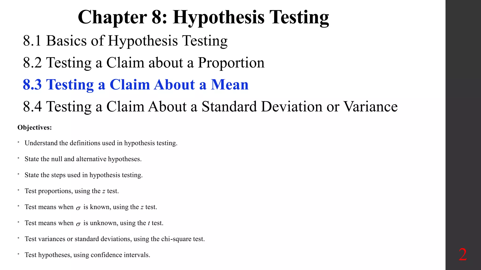
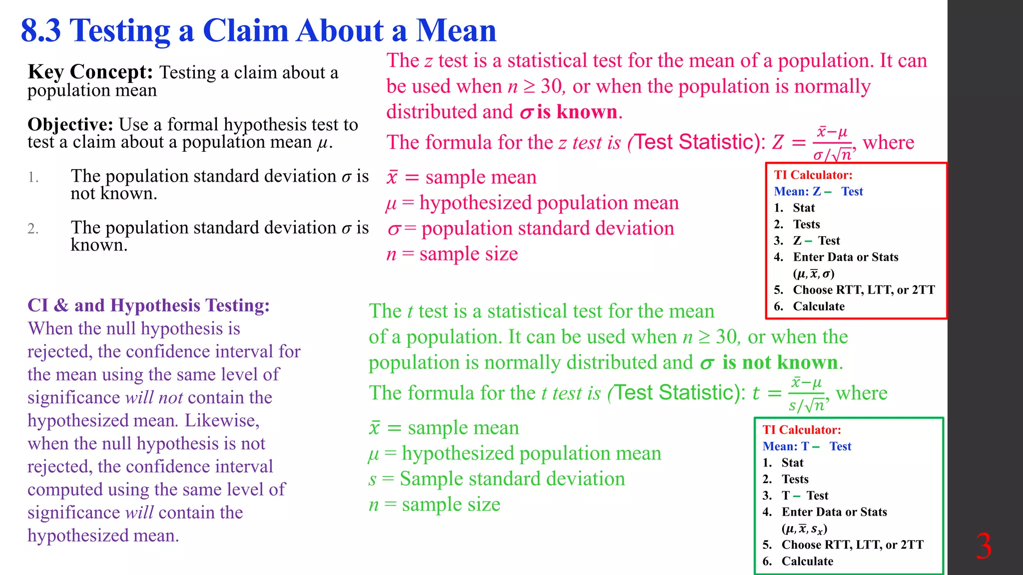
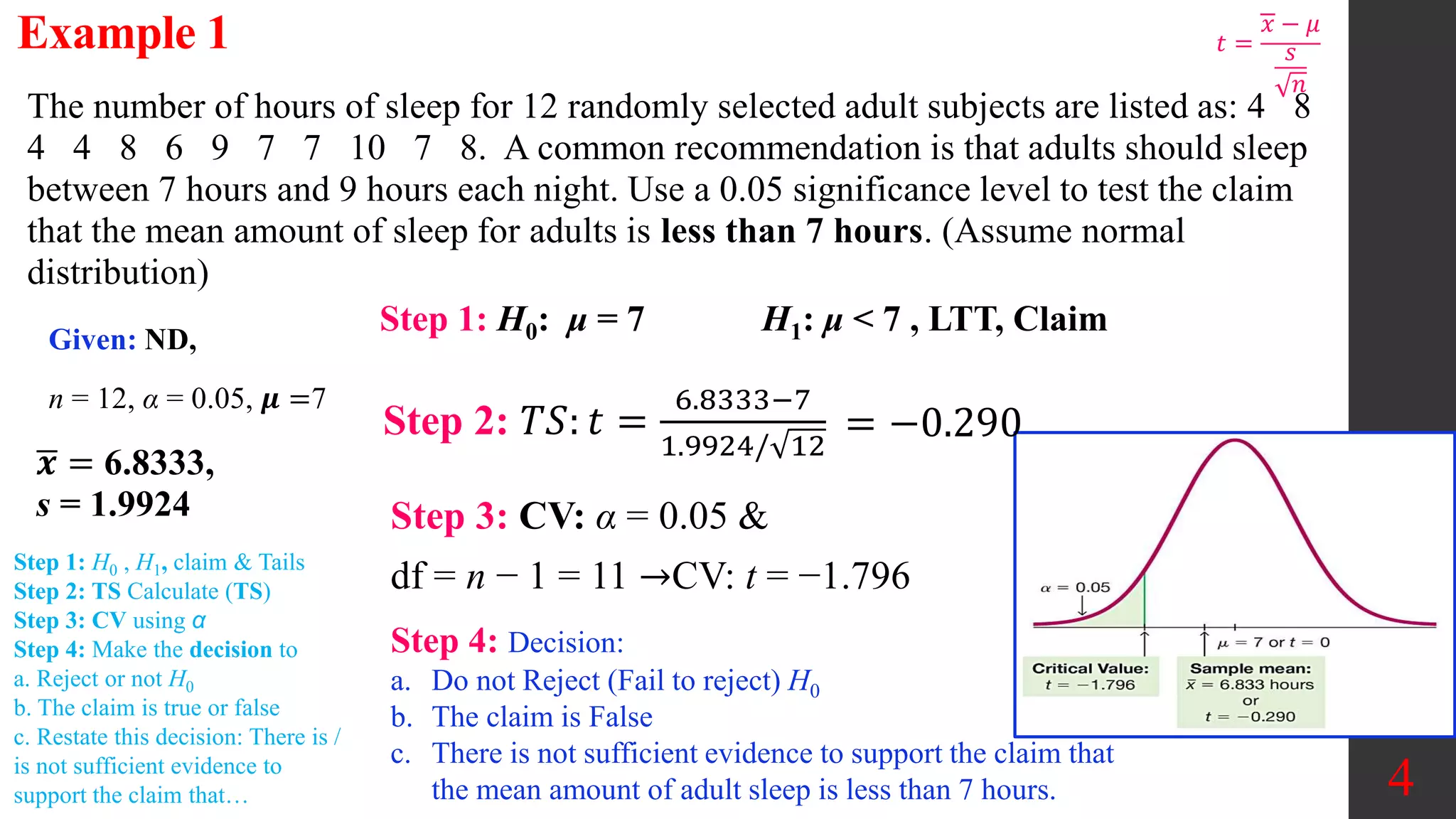
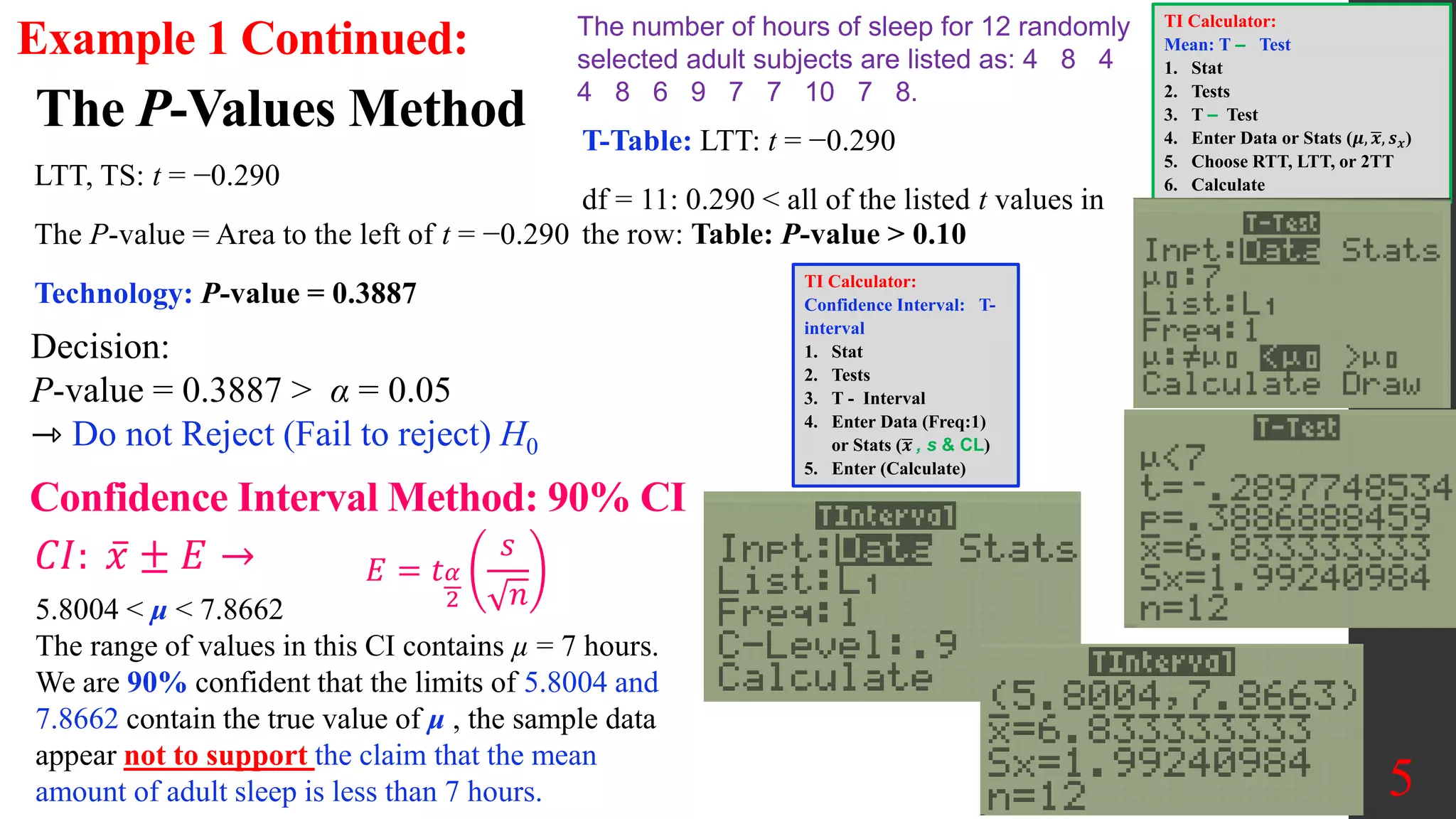
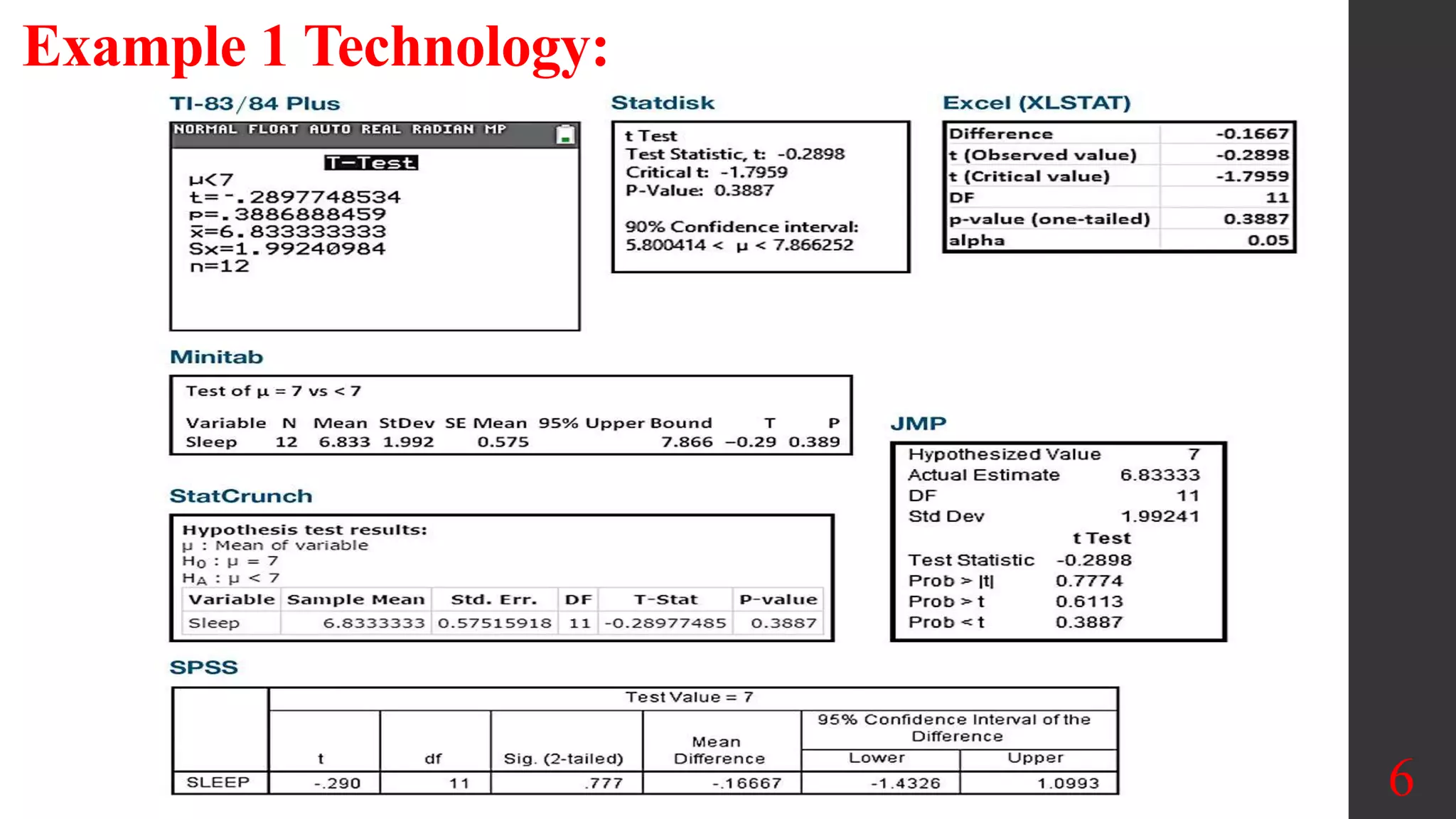
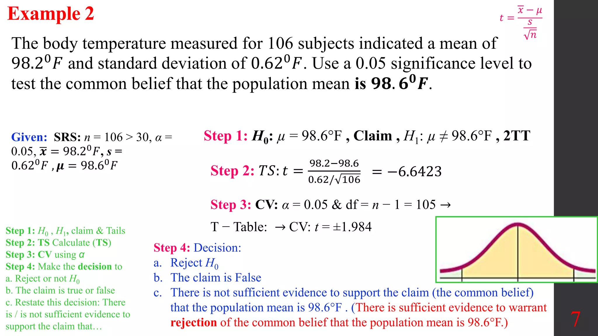
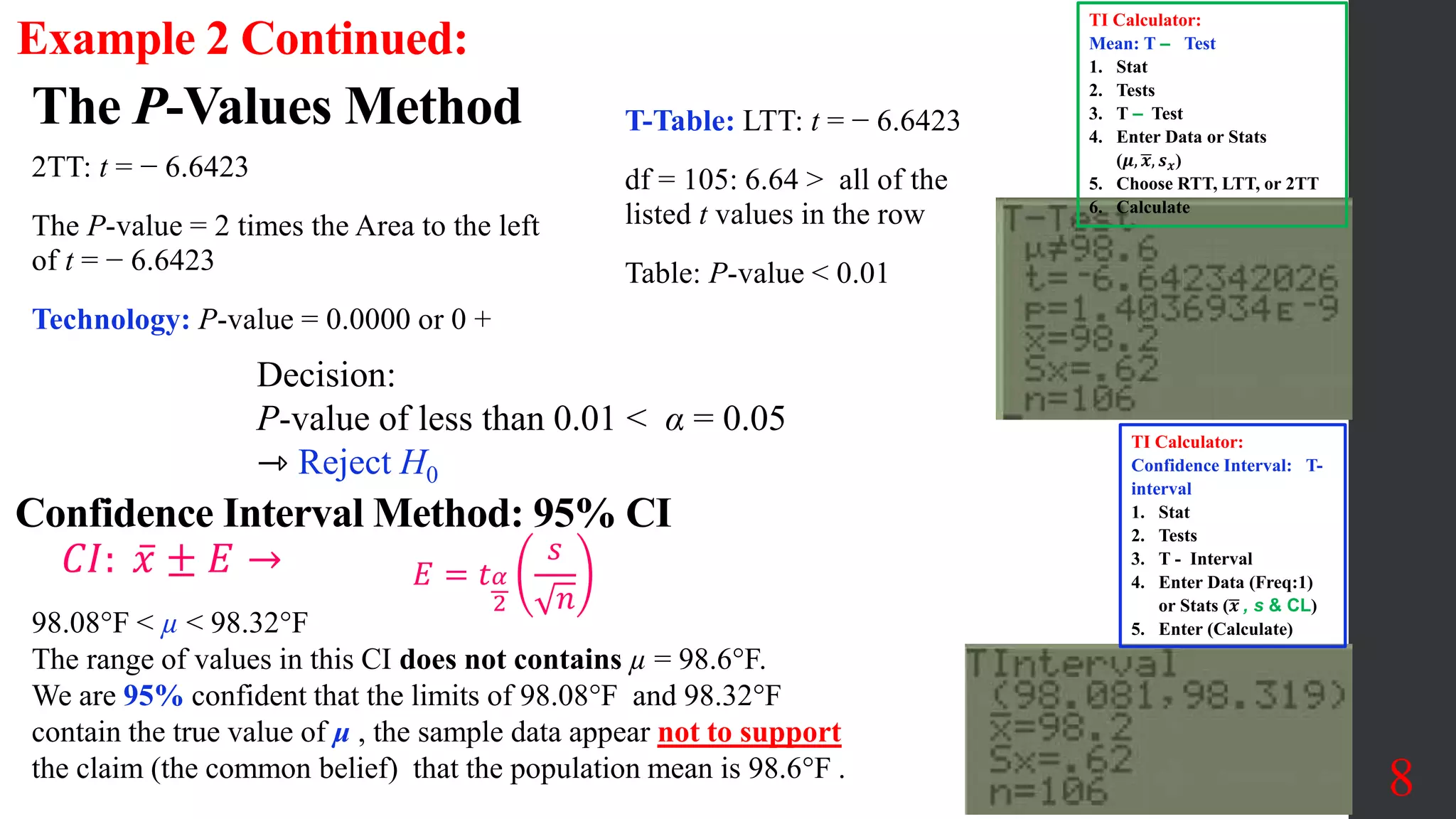
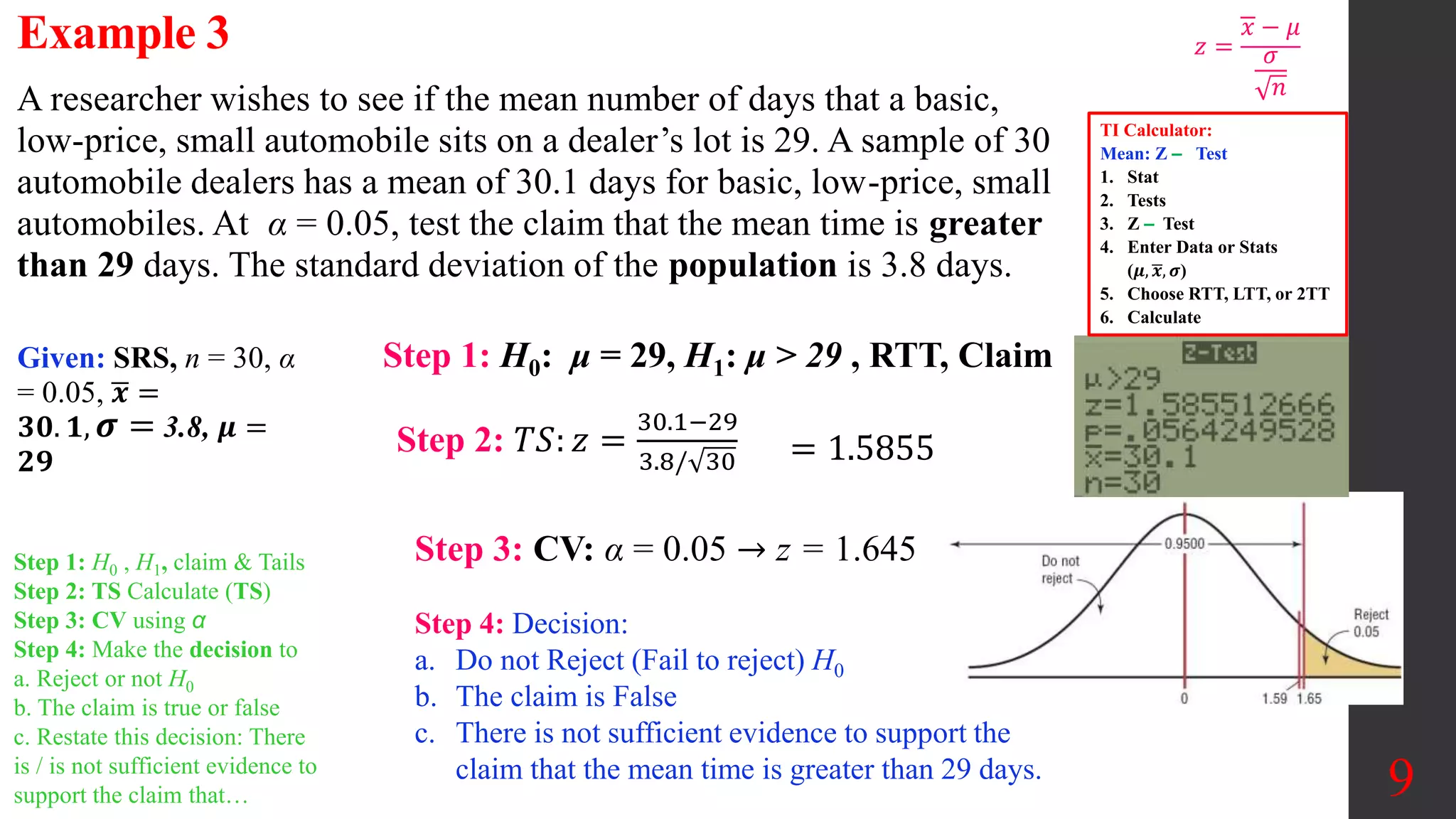
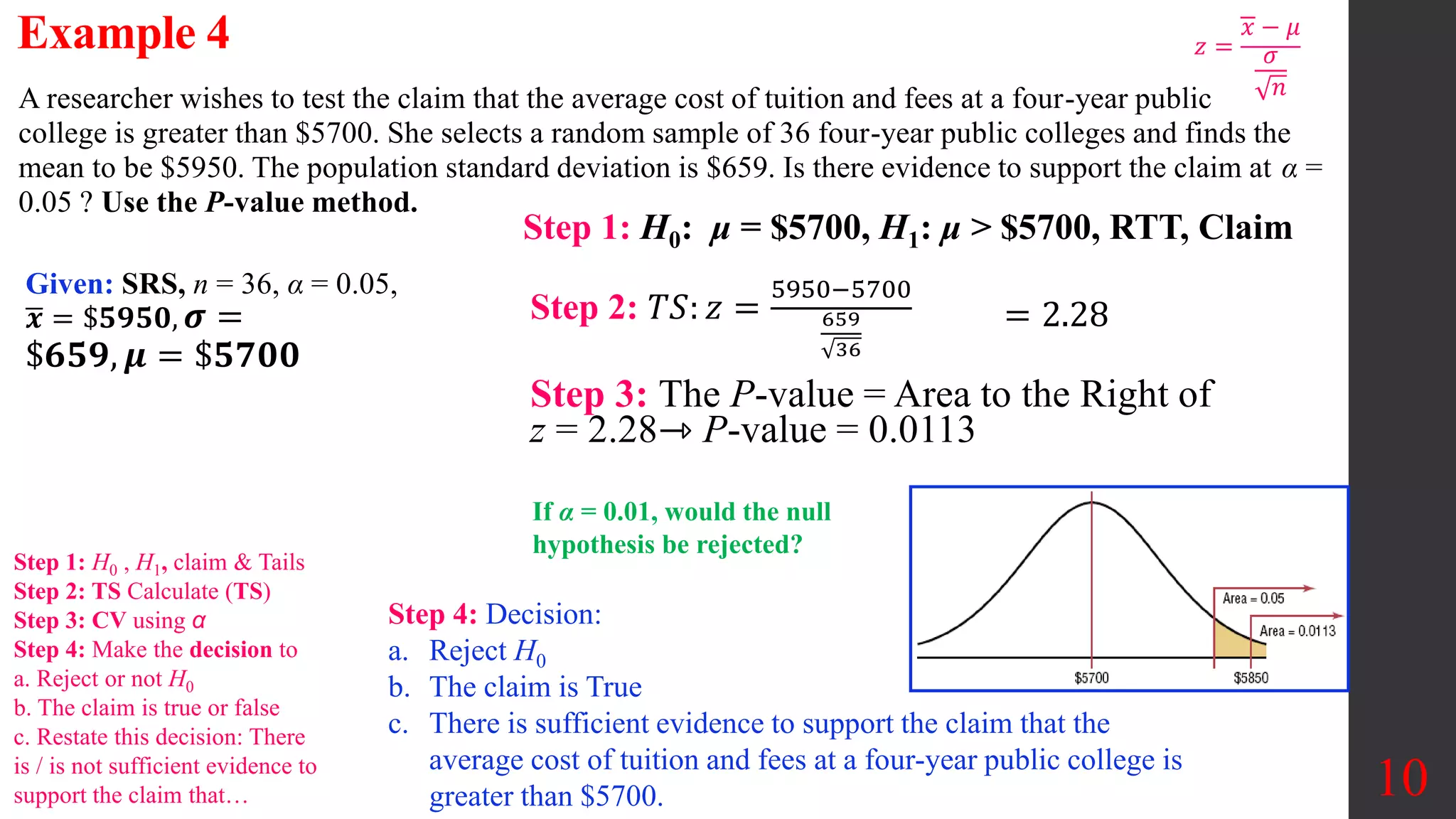
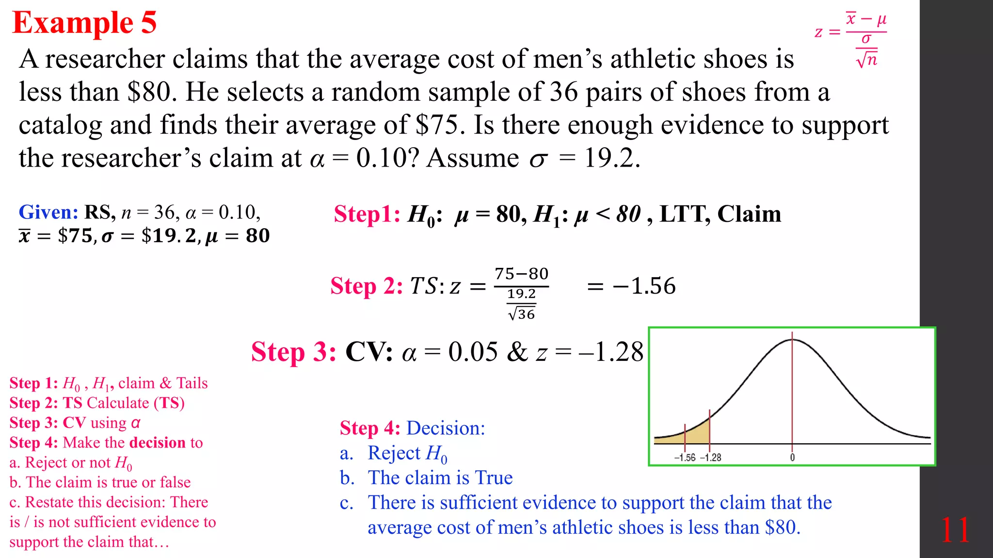
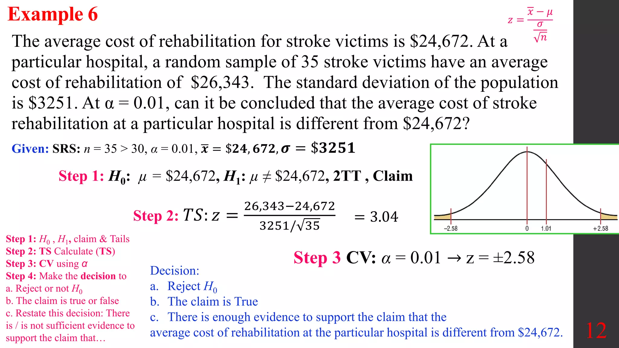
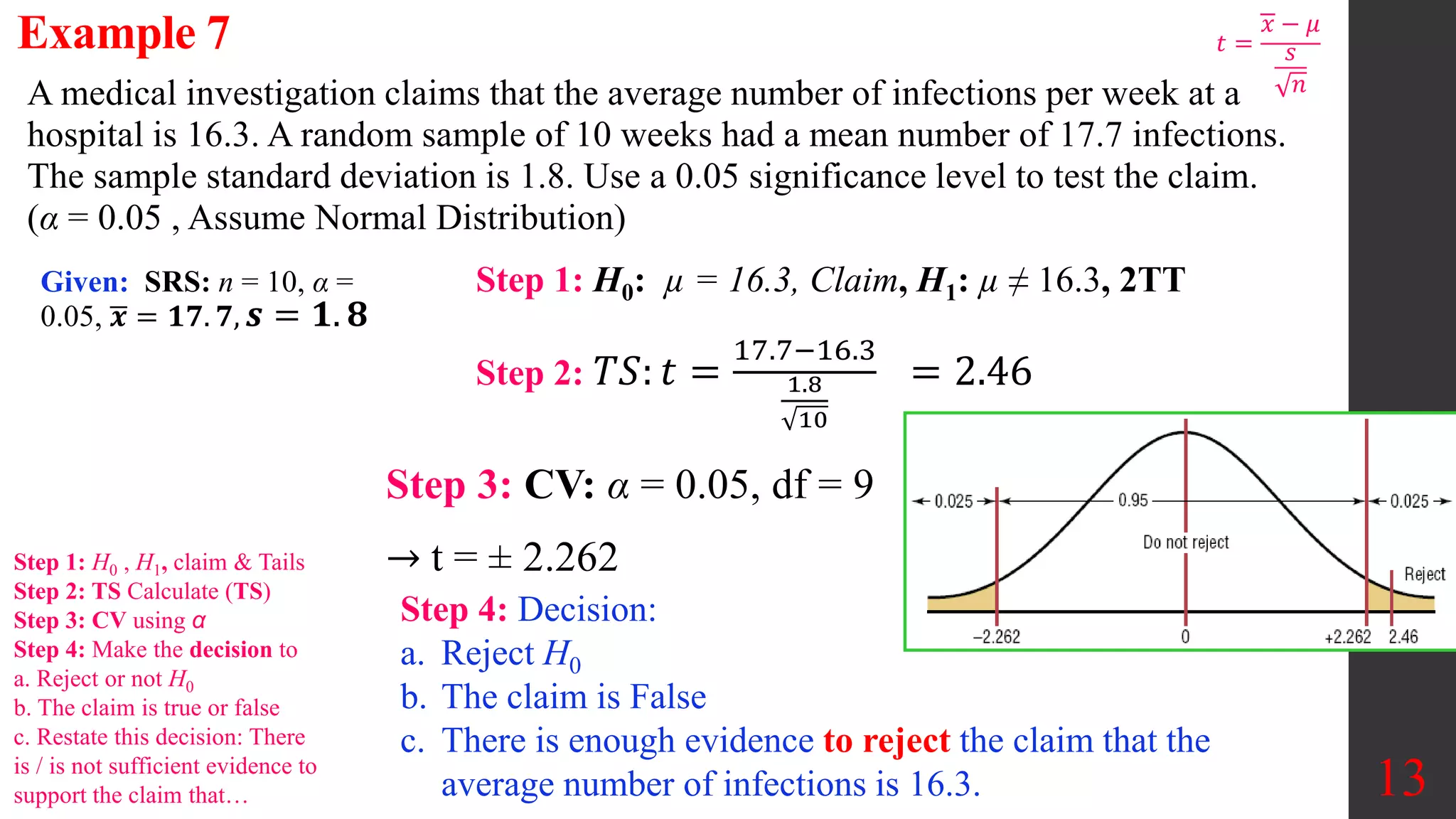
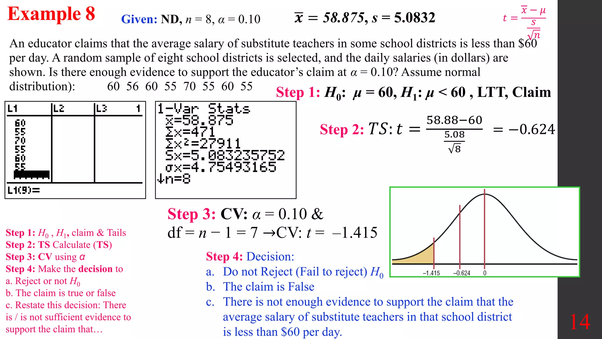
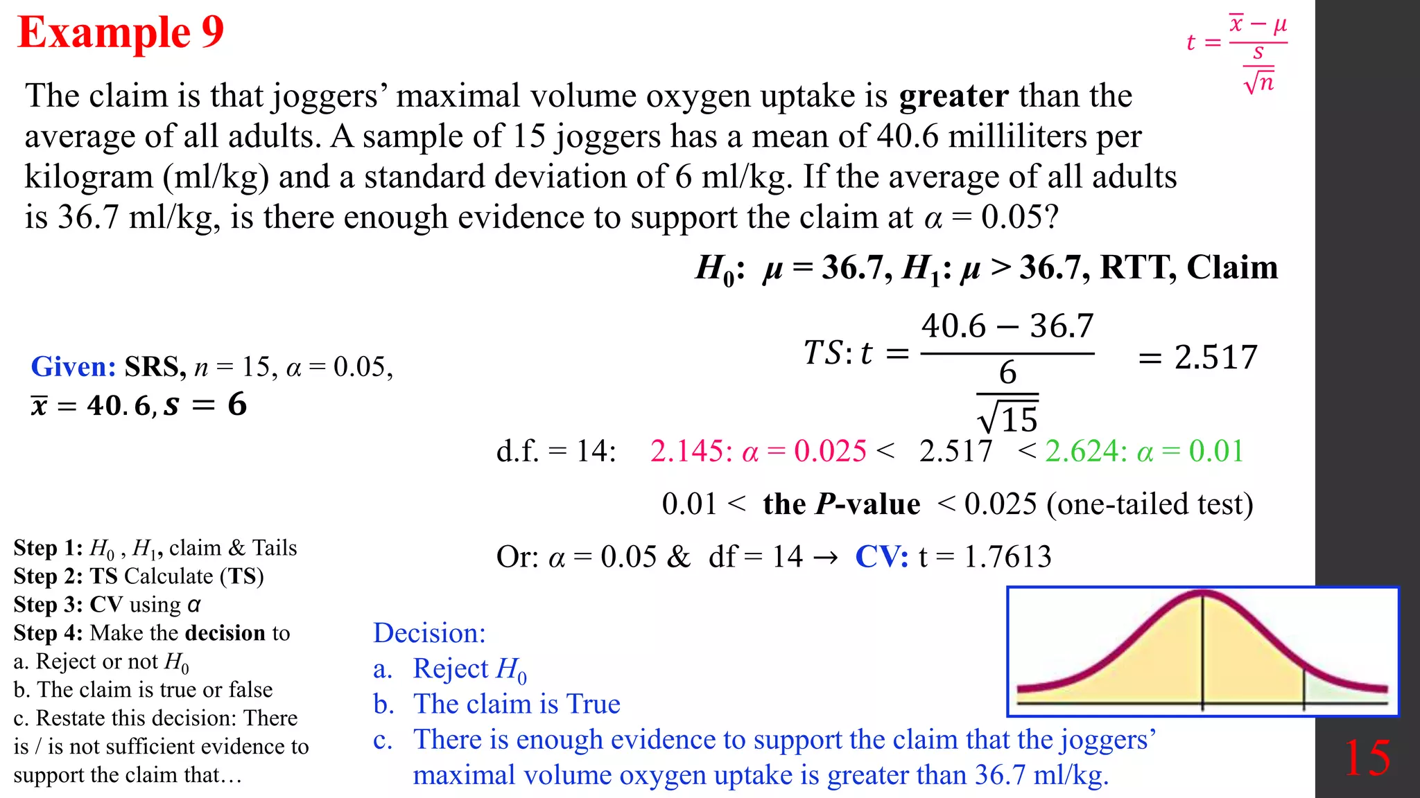
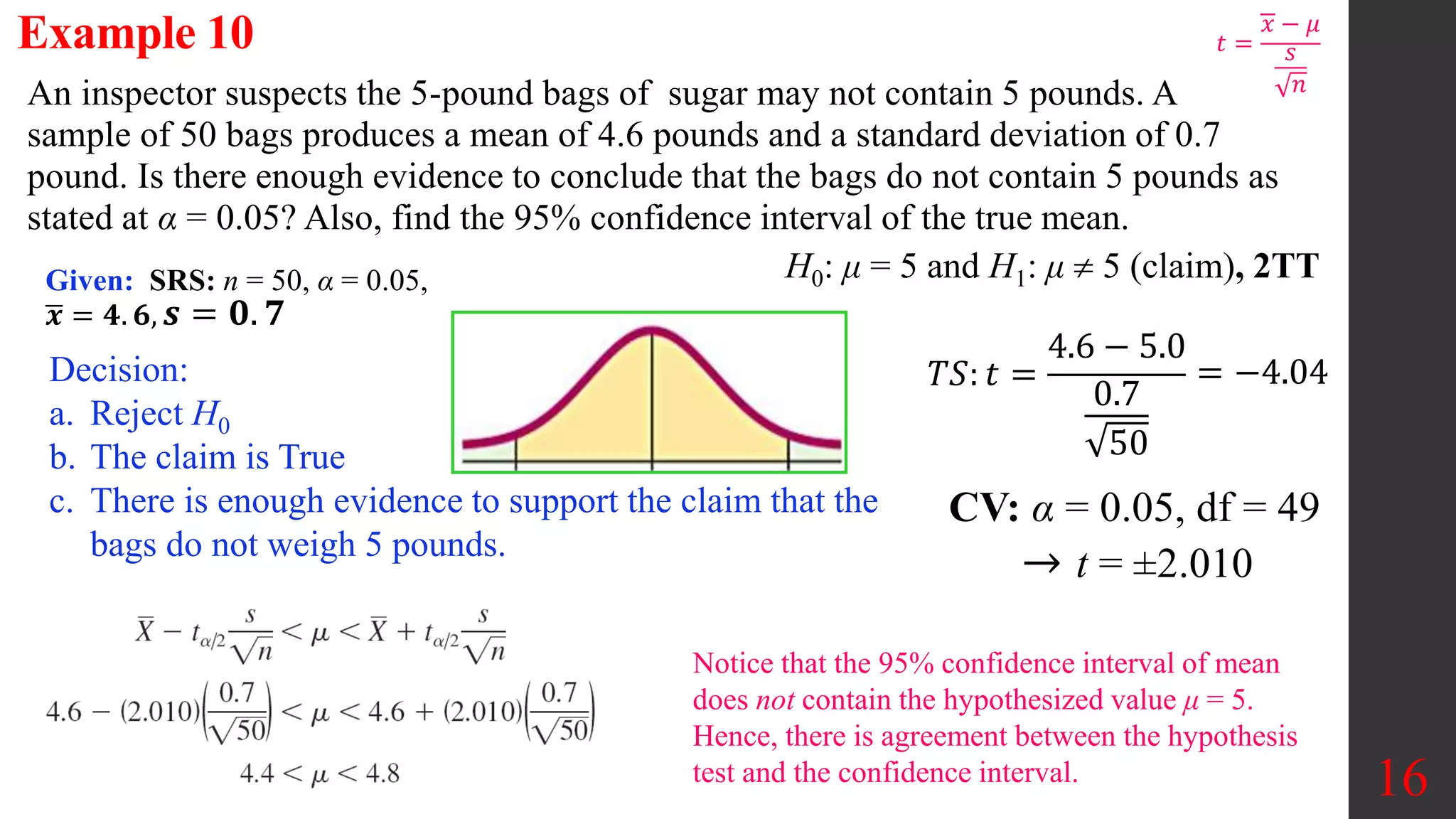
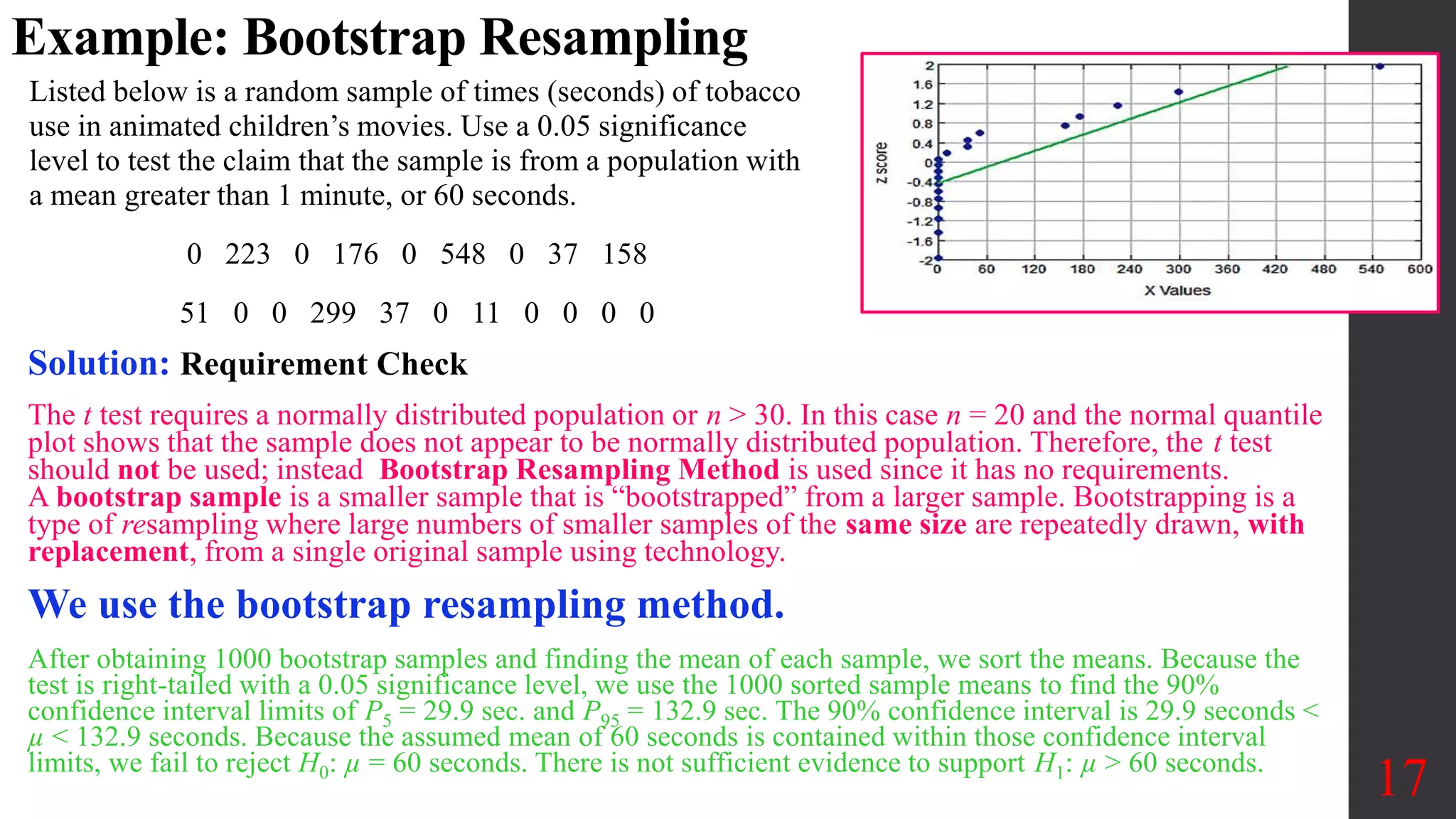

Chapter 8 of Elementary Statistics focuses on hypothesis testing, detailing methods for testing claims about population means, proportions, and standard deviations. It outlines the steps involved in hypothesis testing, including defining null and alternative hypotheses, utilizing z-tests and t-tests, and interpreting p-values and confidence intervals. Several examples illustrate how to apply these statistical tests to real-world scenarios, examining claims around means and providing decisions based on significance levels.