Downloaded 24 times

The document contains statistical analysis problems covering correlation, regression, and hypothesis testing related to various datasets. It provides detailed solutions involving calculations for correlation coefficients, regression equations, goodness-of-fit tests, and tests of independence and homogeneity, explaining the methods and decision-making processes for each statistical test. Key results include determining whether variables are related or independent, with specific emphasis on how testosterone affects metabolic rates and claims about category proportions in different scenarios.
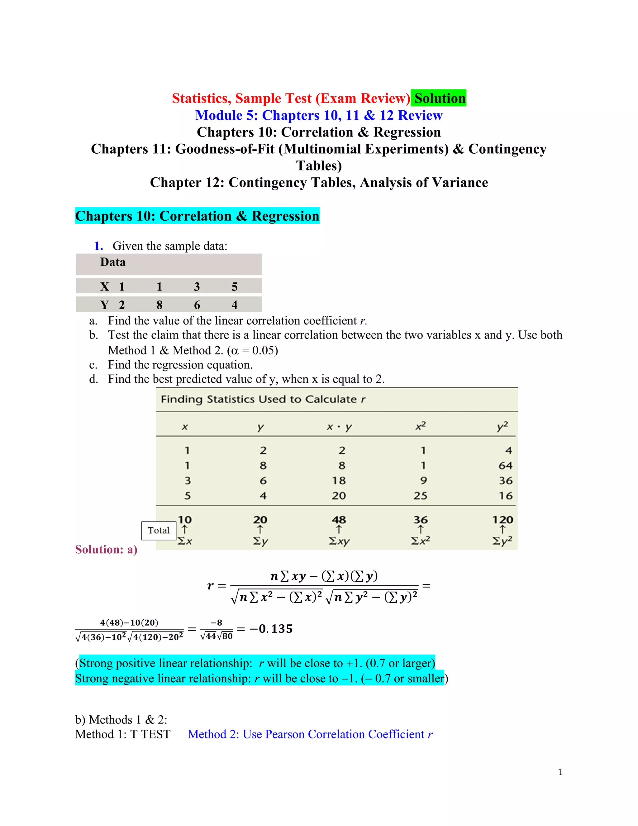
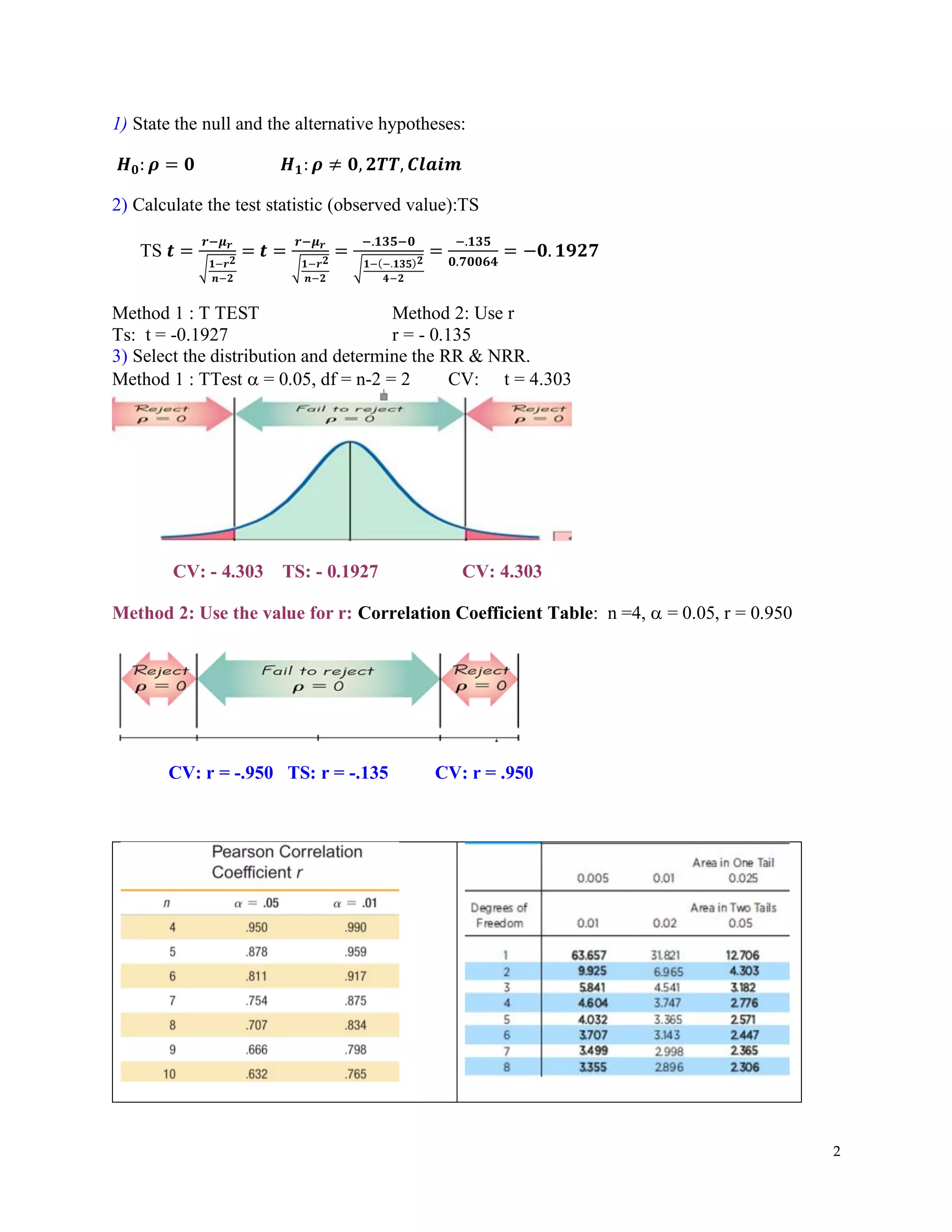
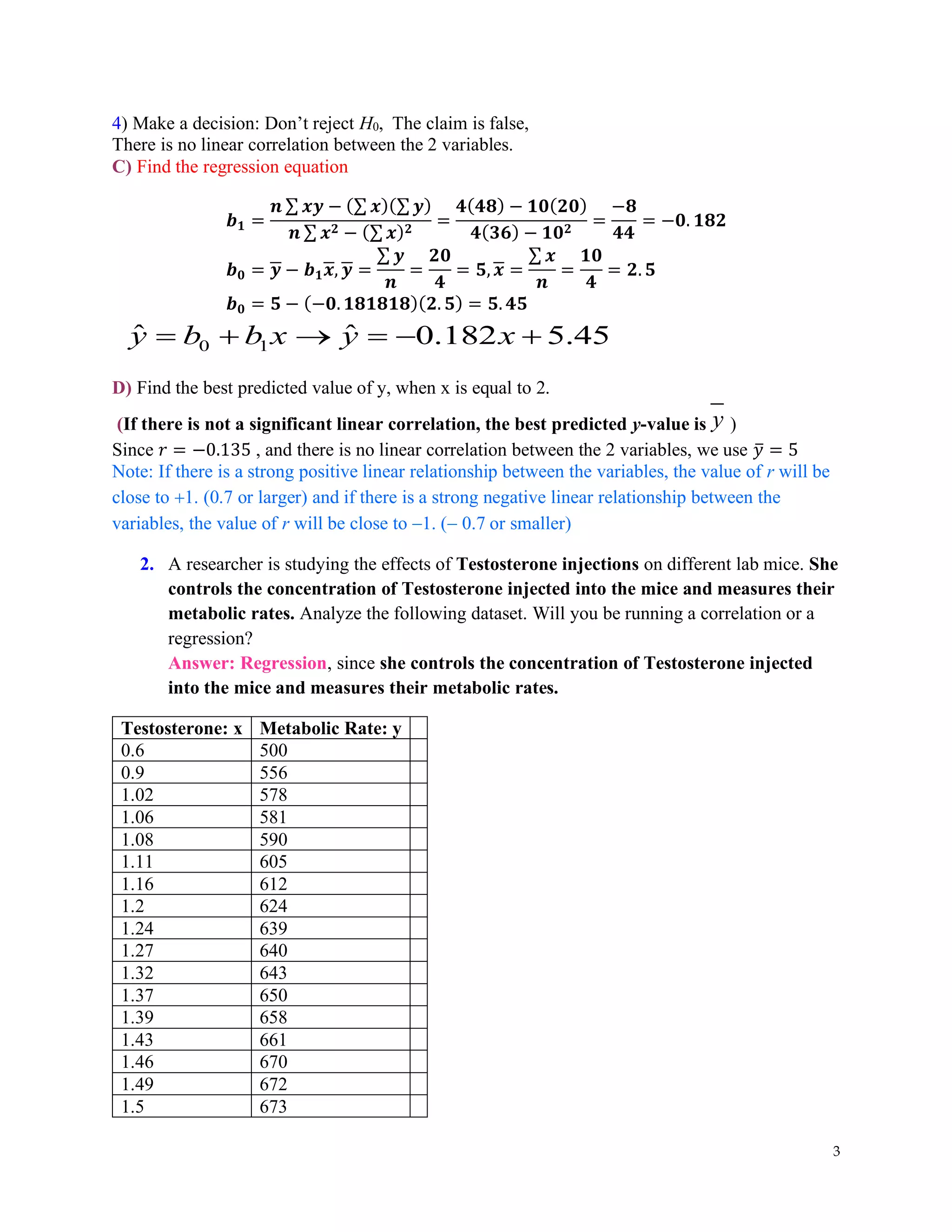
Discusses linear correlation coefficient and regression equations using sample data.
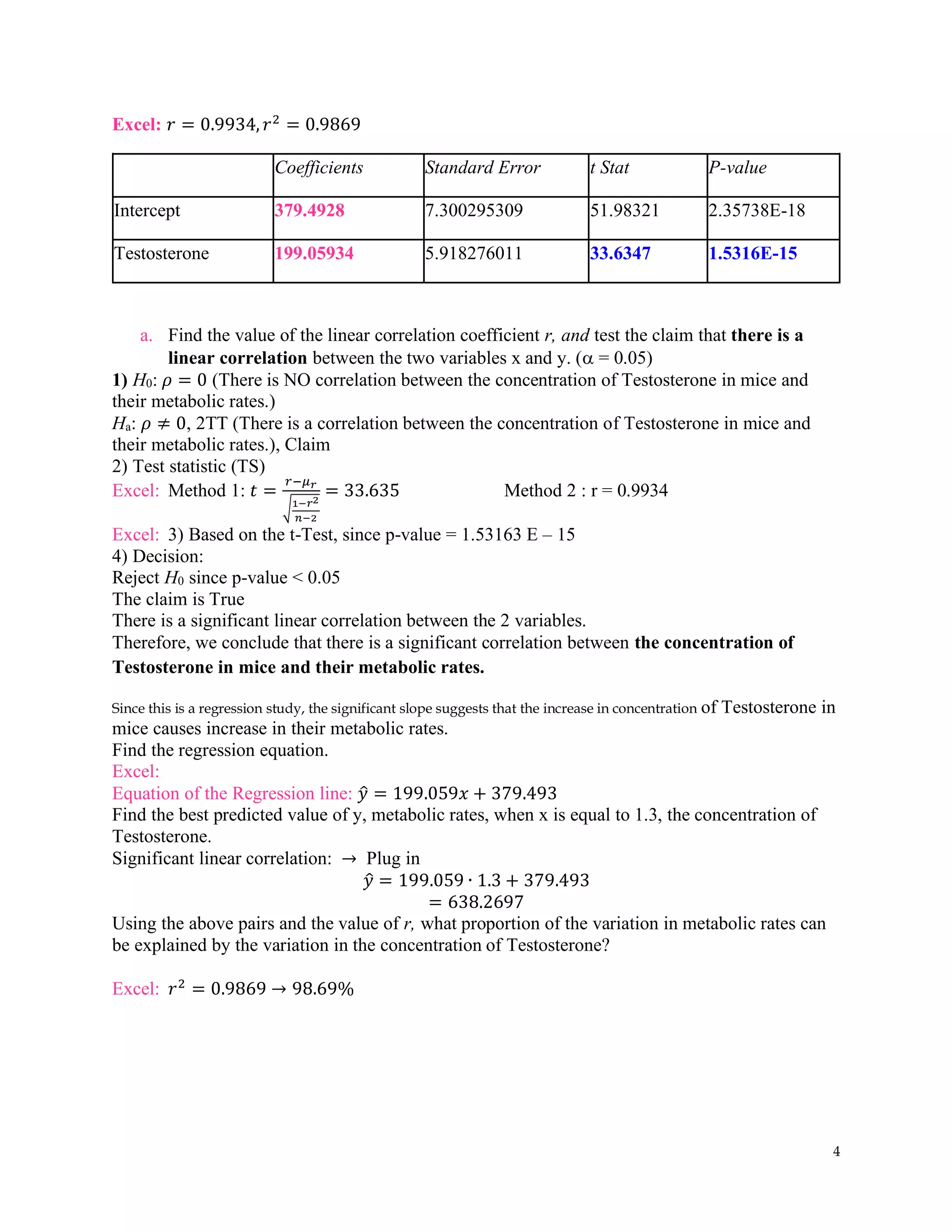
Analyzes the correlation and regression between testosterone levels and metabolic rates in mice.
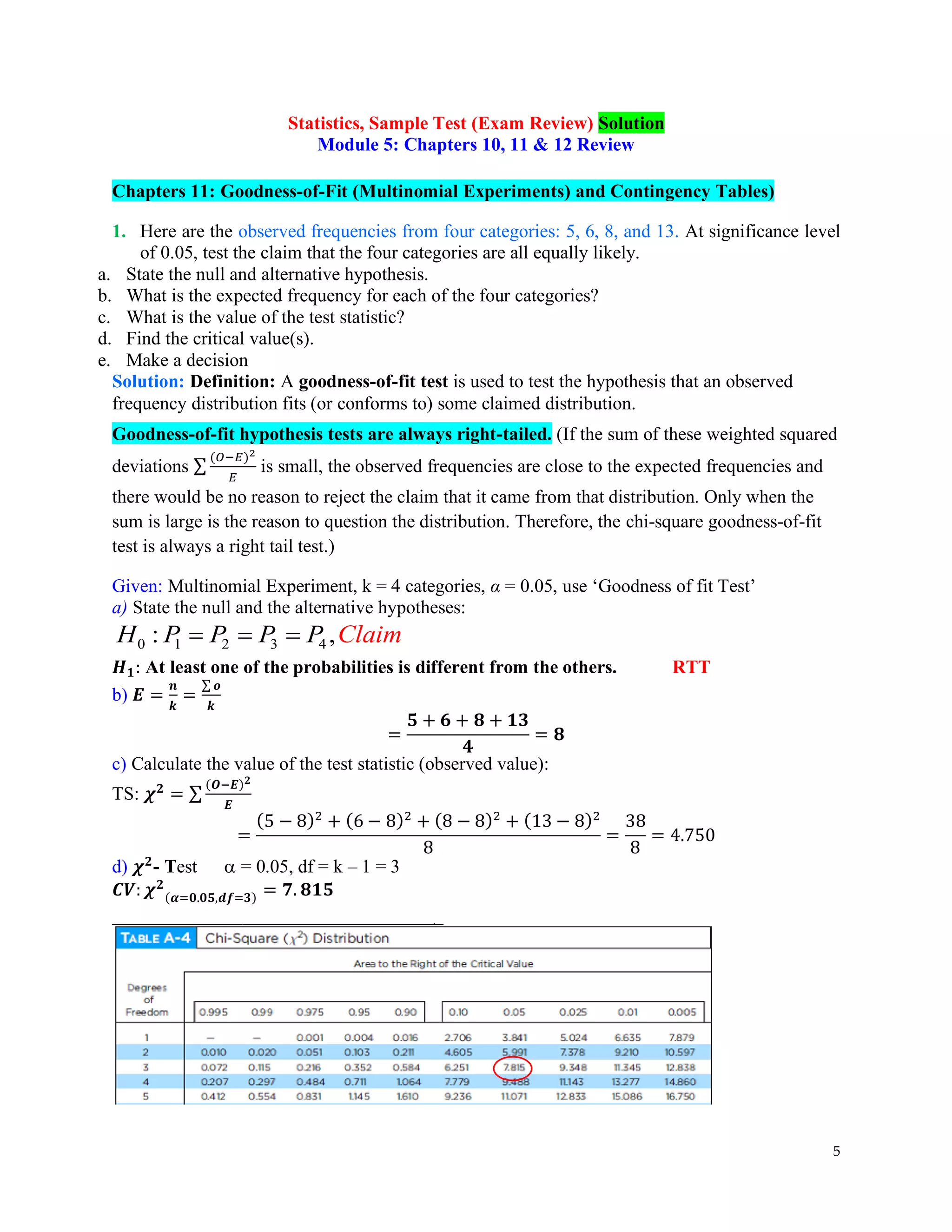
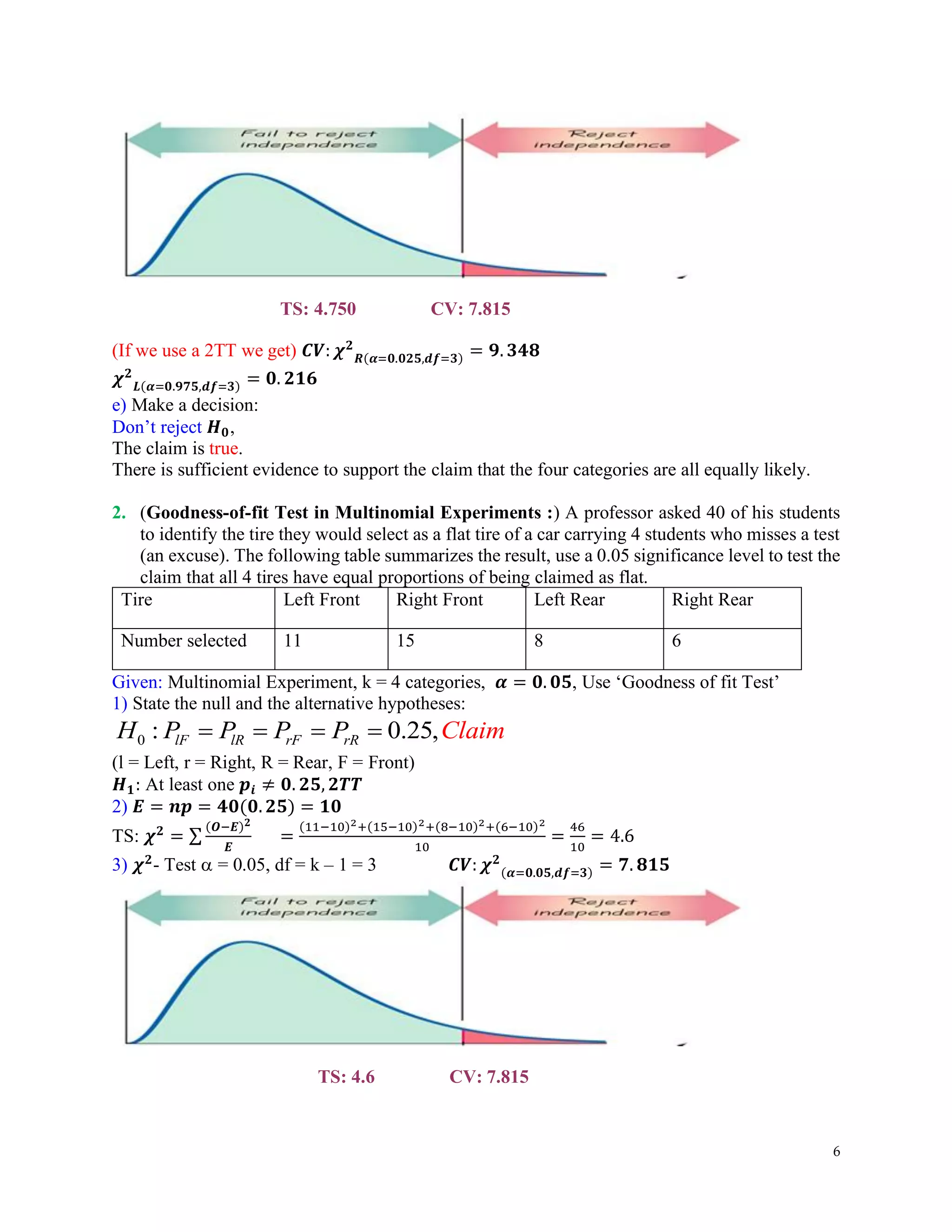
Tests the equality of observed frequencies across multiple categories, using chi-square tests.Continuation of goodness-of-fit tests using different experiments to compare observed against expected.
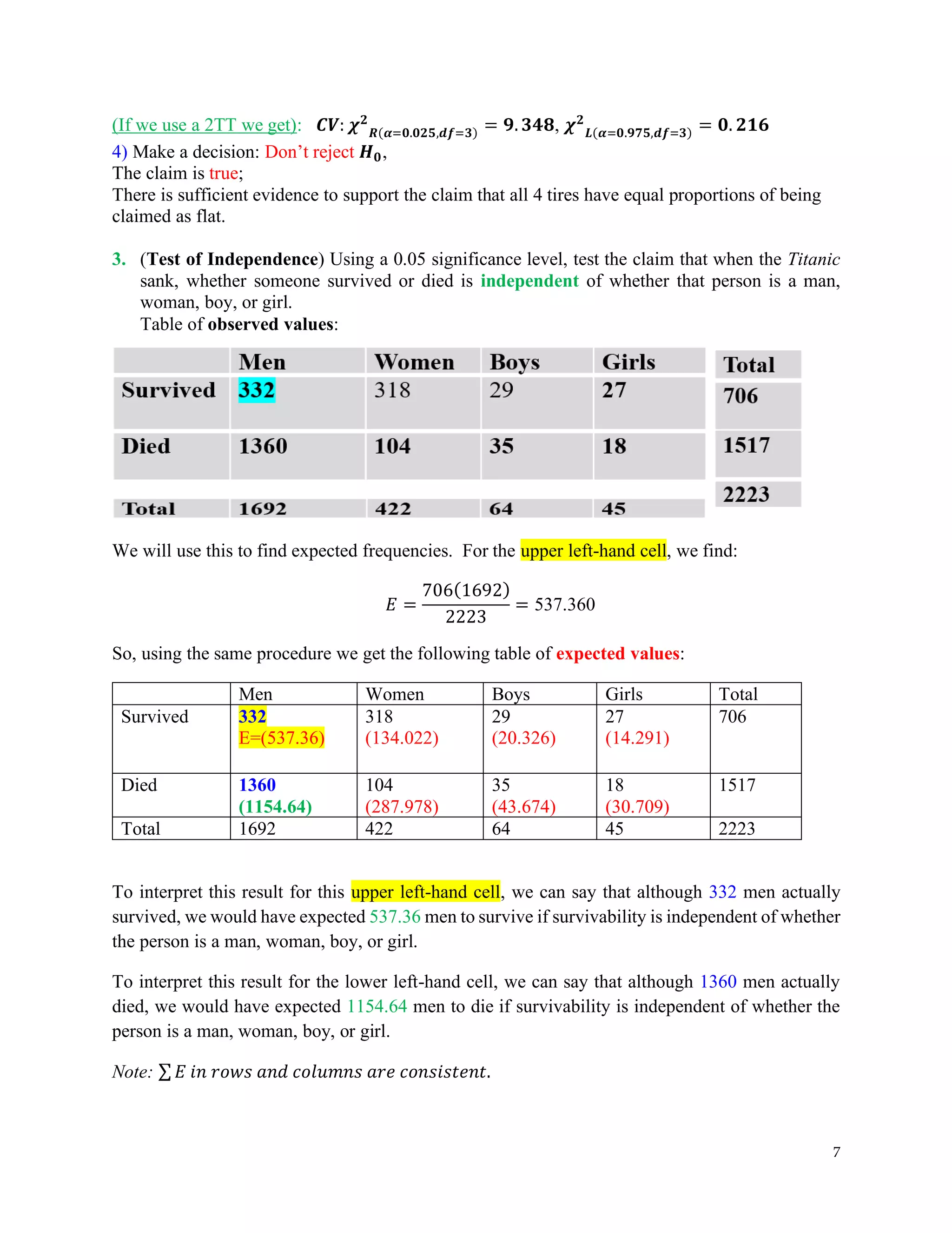
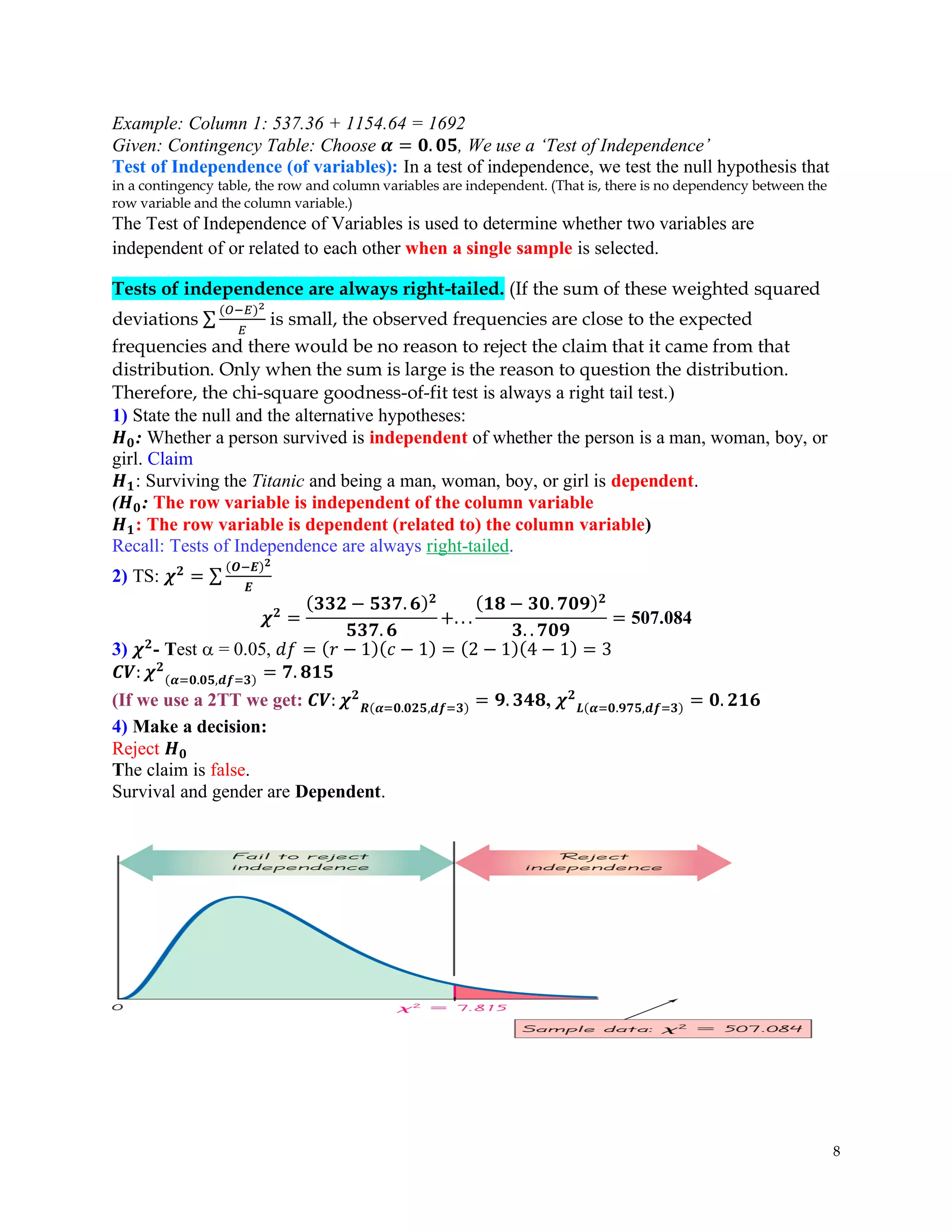
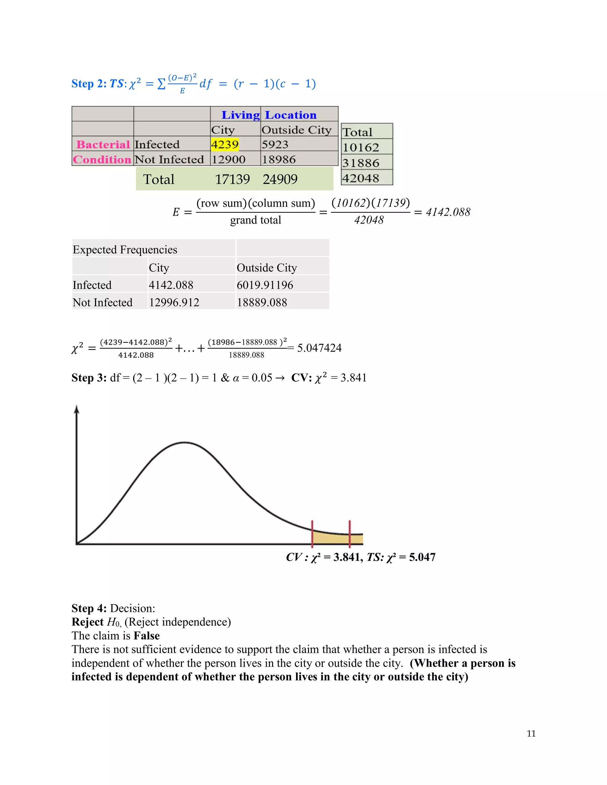
Discusses the use of contingency tables to test whether two variables (survival and gender) are independent.
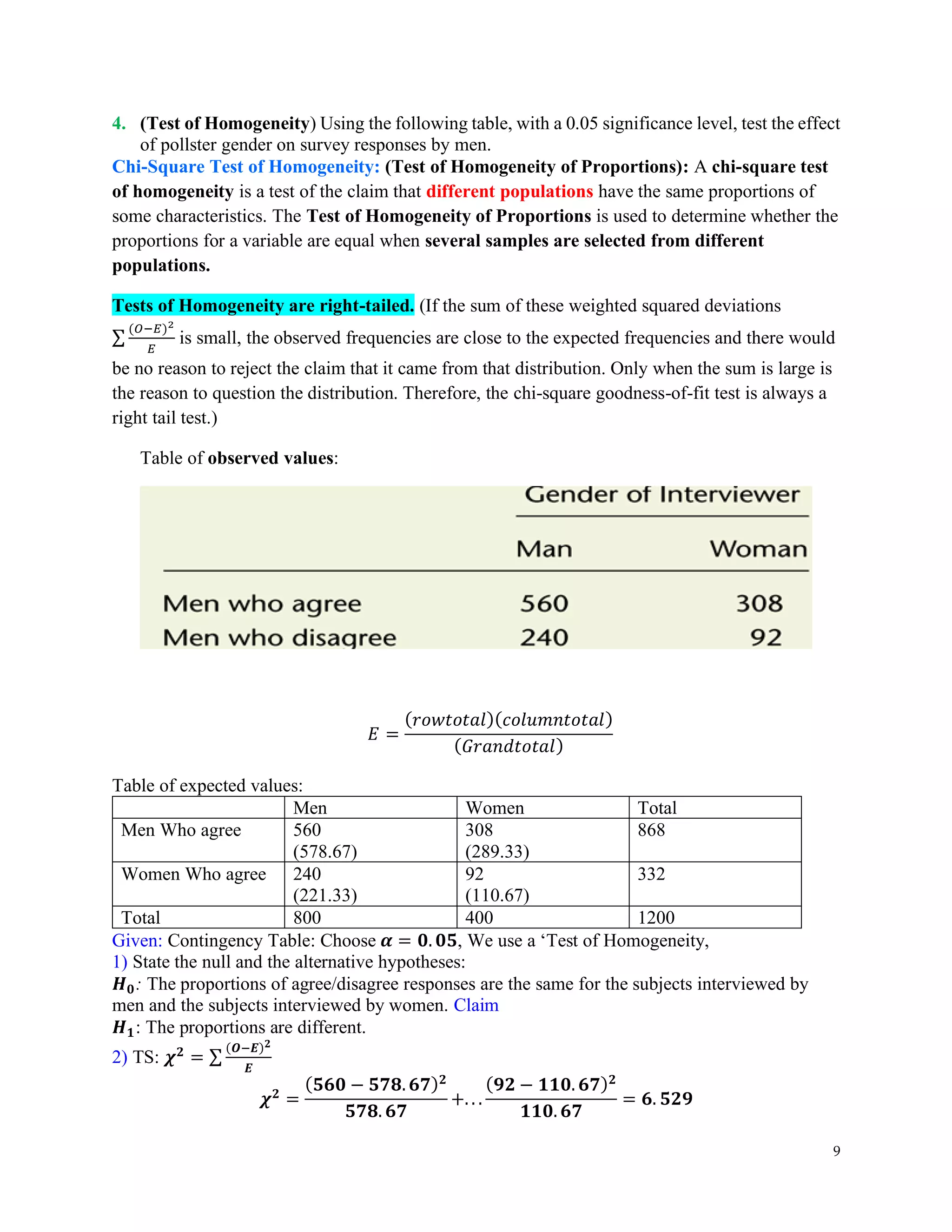
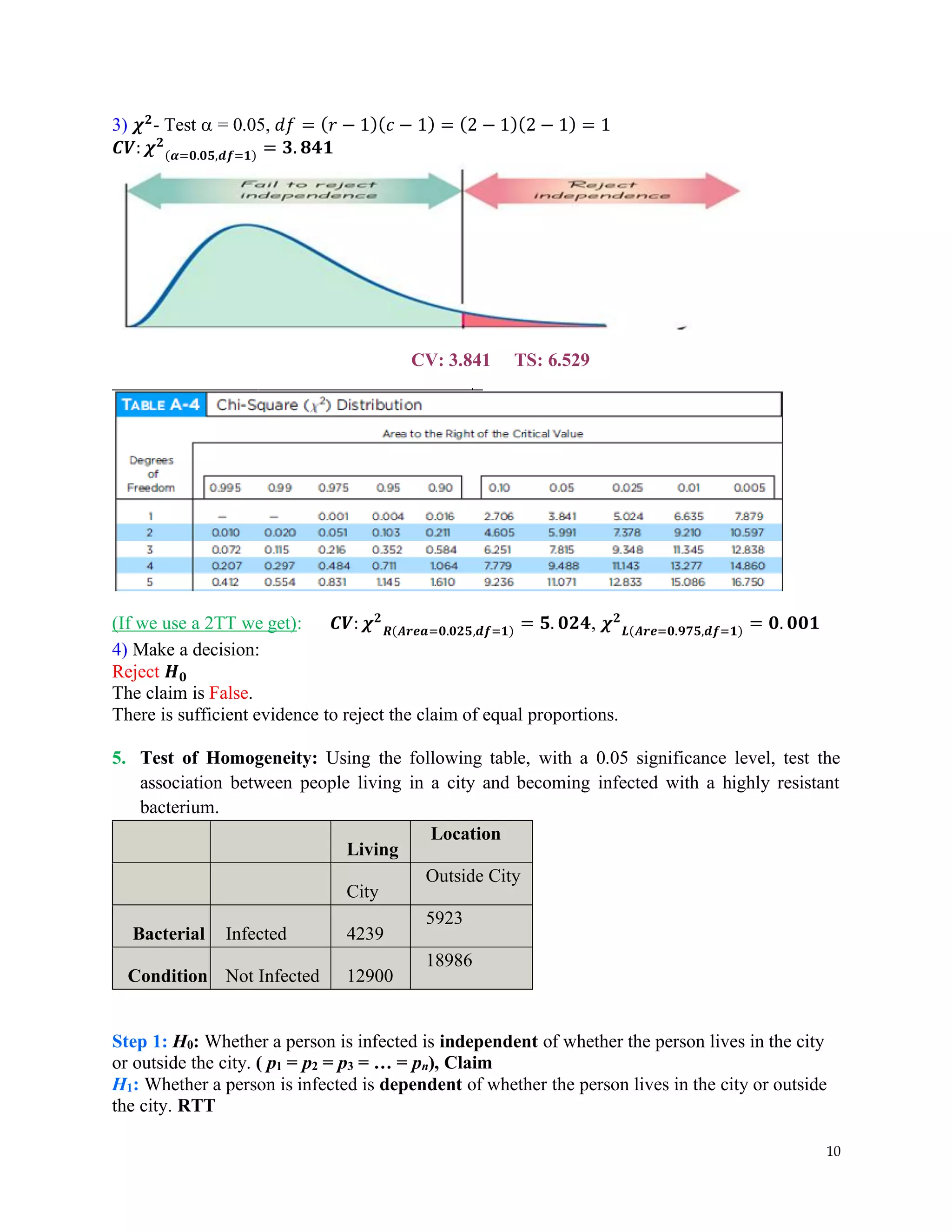
Evaluates agreement proportions between different groups using chi-square tests of homogeneity.
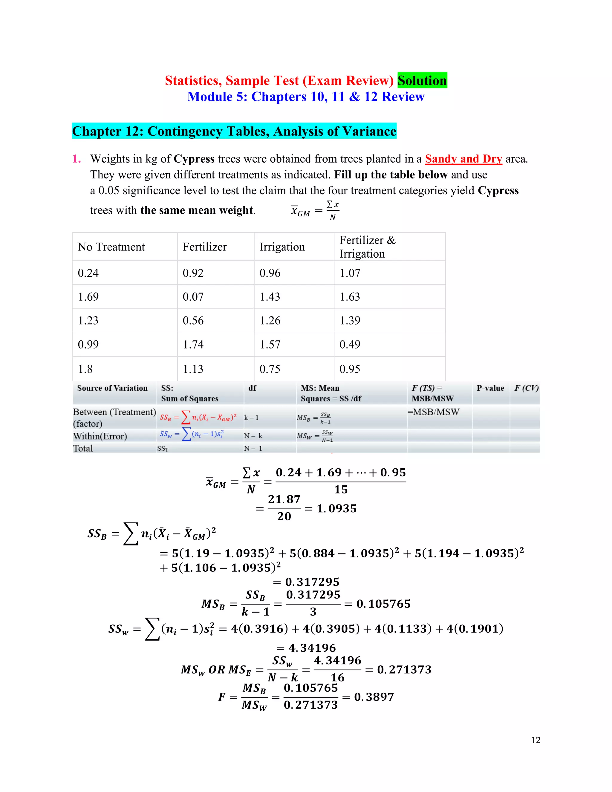
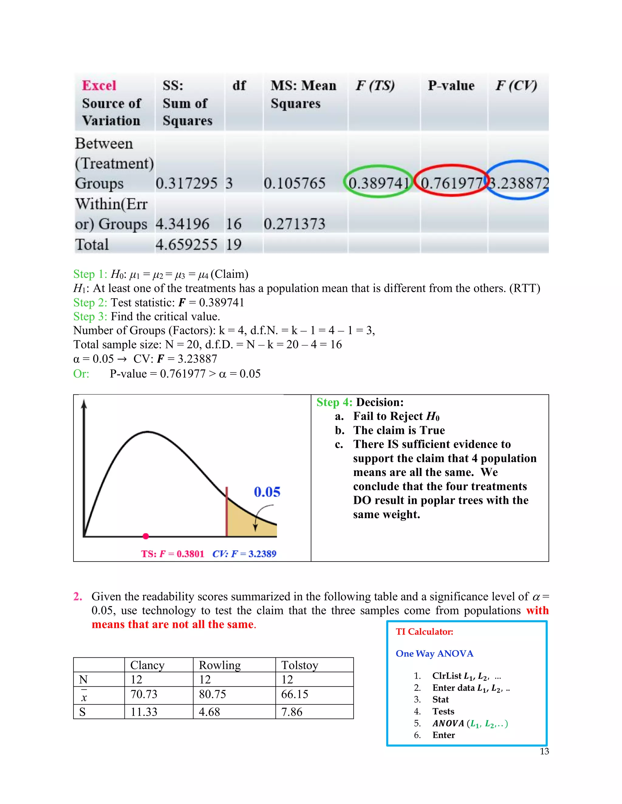
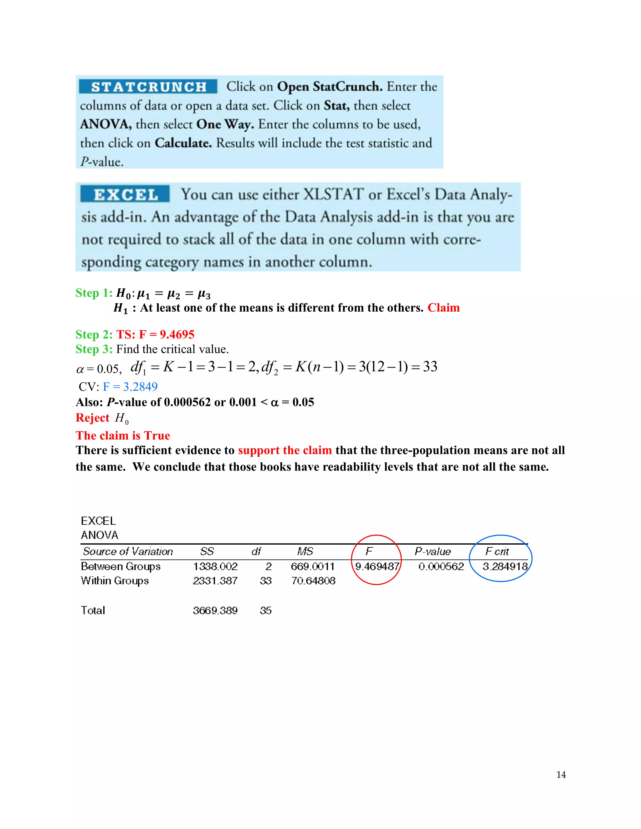
Uses ANOVA to analyze weight differences among Cypress trees under various treatments.