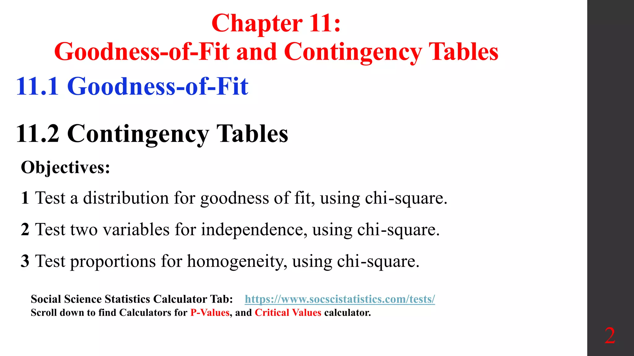
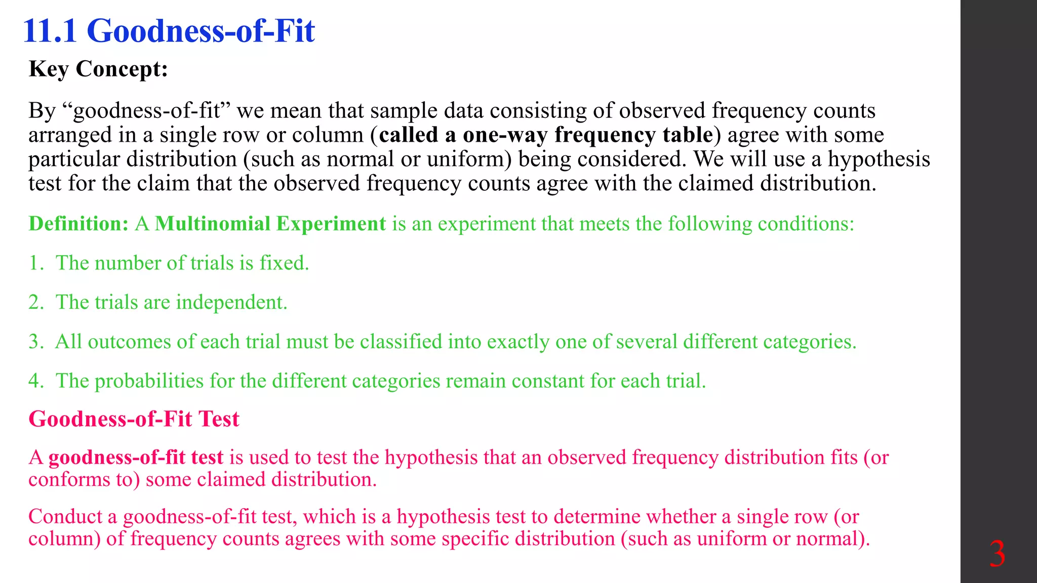
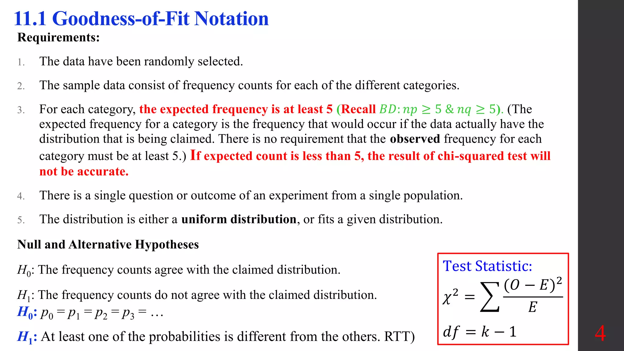
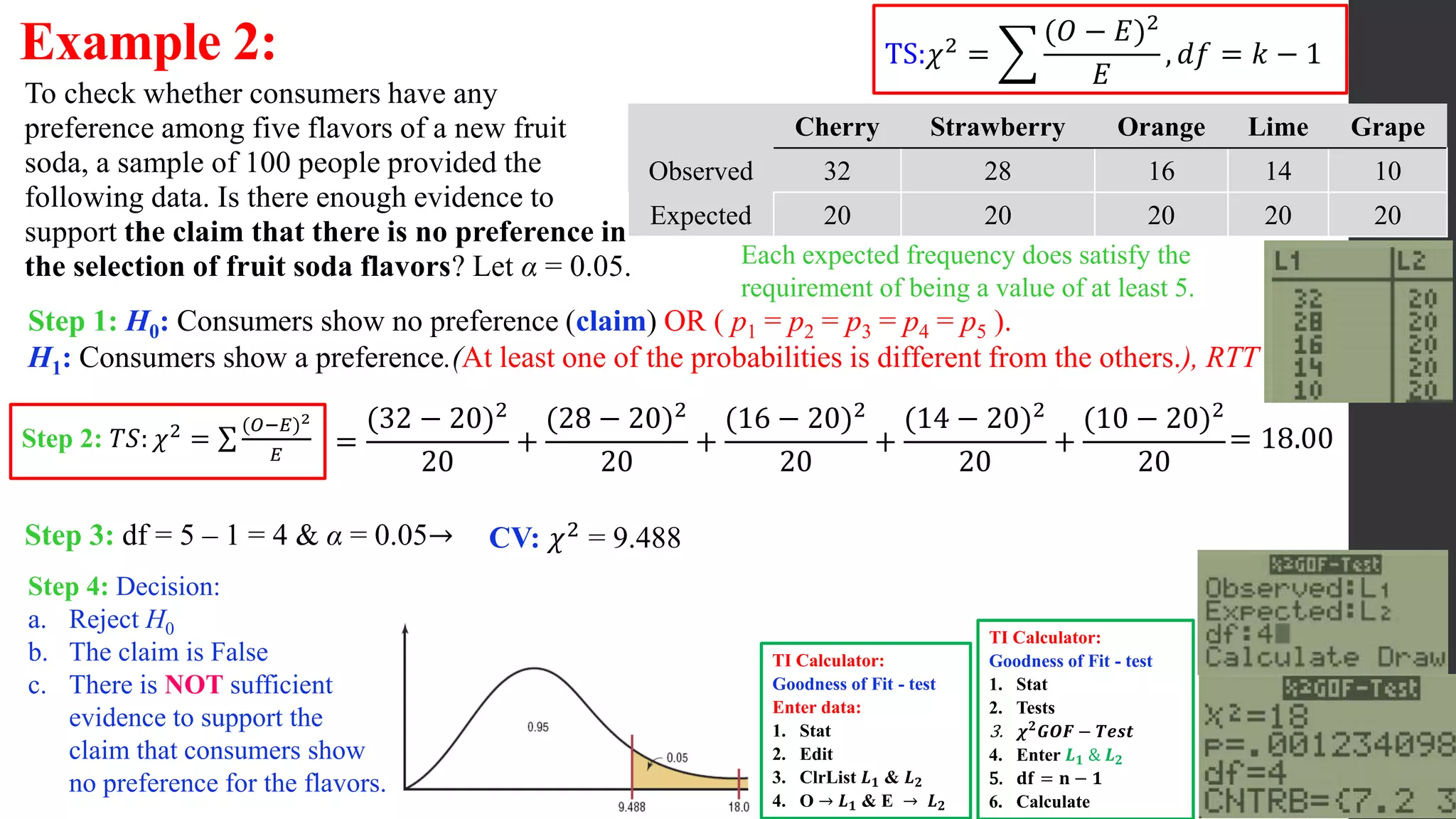
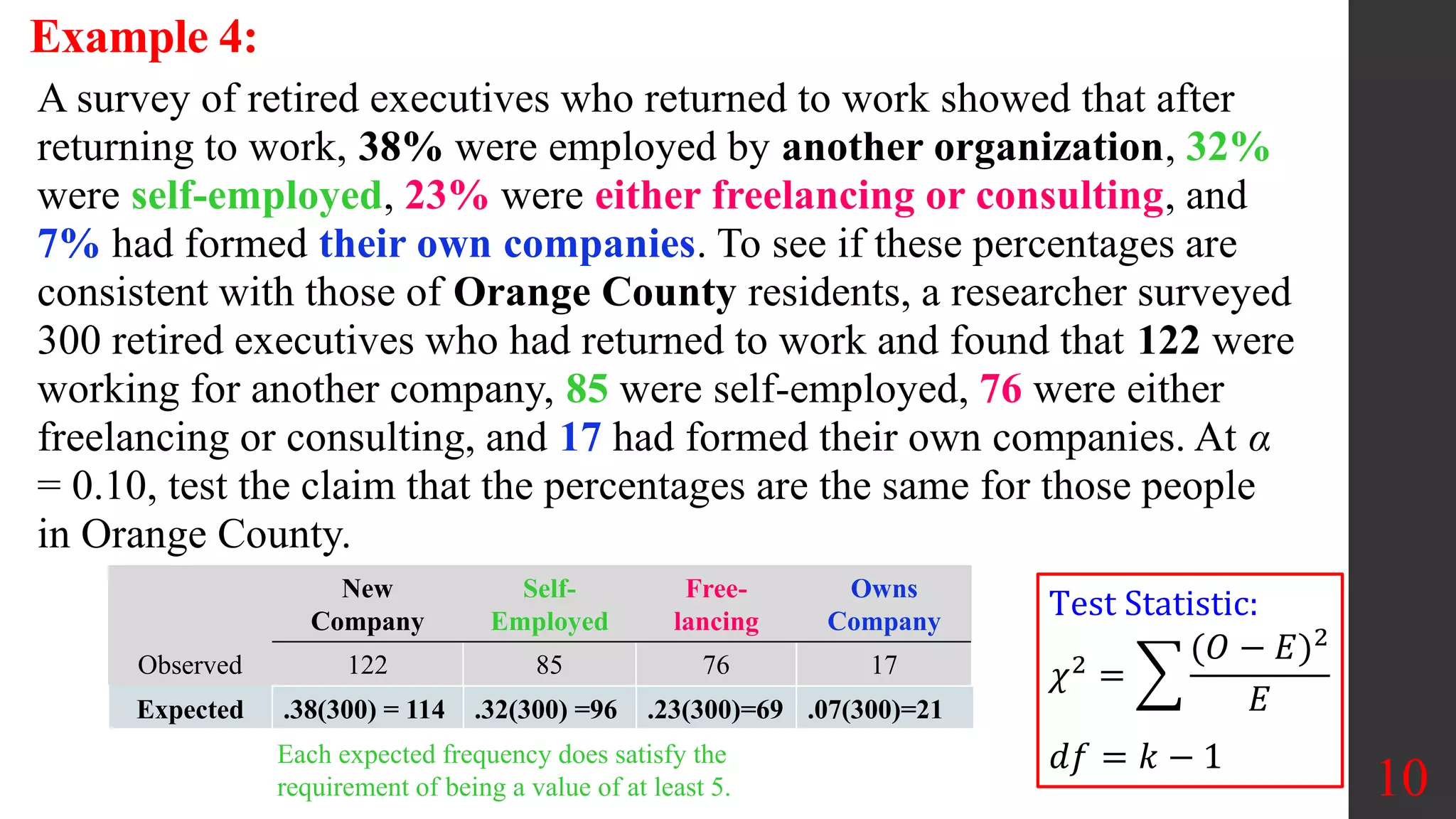
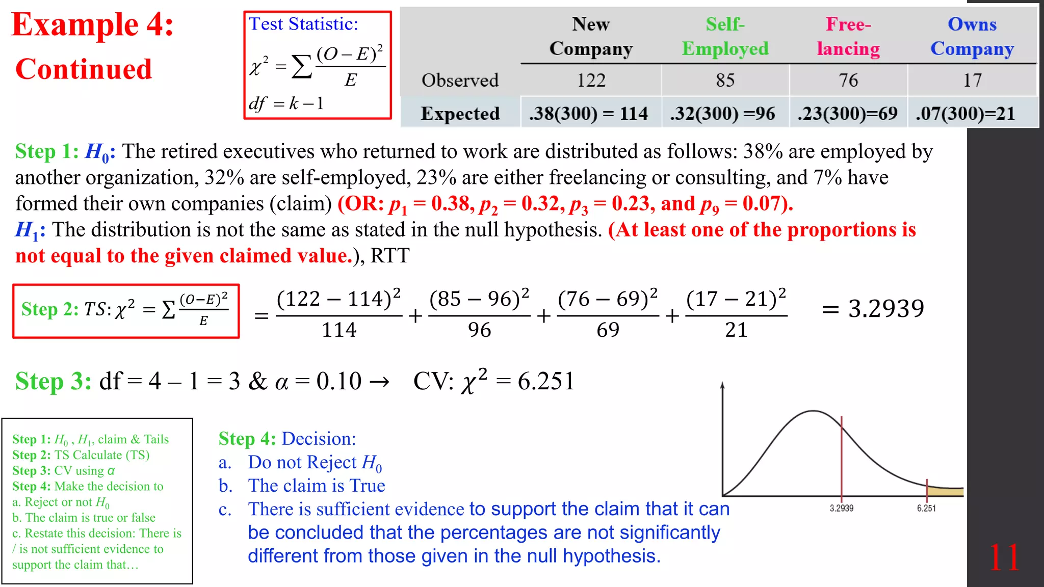
The document provides information about goodness-of-fit tests and contingency tables. It defines a goodness-of-fit test as testing whether an observed frequency distribution fits a claimed distribution. It also provides the notation, requirements, and steps to conduct a goodness-of-fit test including: defining the null and alternative hypotheses, calculating the test statistic as a chi-square value, finding the critical value, and making a decision to reject or fail to reject the null hypothesis. Several examples demonstrate how to perform goodness-of-fit tests to determine if sample data fits a claimed distribution.

1. Elementary Statistics
Chapter 11:
Goodness-of-Fit and
Contingency Tables
11.1 Goodness-of-Fit
1

2. Chapter 11:
Goodness-of-Fit and Contingency Tables
11.1 Goodness-of-Fit
11.2 Contingency Tables
2
Objectives:
1 Test a distribution for goodness of fit, using chi-square.
2 Test two variables for independence, using chi-square.
3 Test proportions for homogeneity, using chi-square.
Social Science Statistics Calculator Tab: https://www.socscistatistics.com/tests/
Scroll down to find Calculators for P-Values, and Critical Values calculator.

3. 3
11.1 Goodness-of-Fit
Key Concept:
By “goodness-of-fit” we mean that sample data consisting of observed frequency counts
arranged in a single row or column (called a one-way frequency table) agree with some
particular distribution (such as normal or uniform) being considered. We will use a hypothesis
test for the claim that the observed frequency counts agree with the claimed distribution.
Definition: A Multinomial Experiment is an experiment that meets the following conditions:
1. The number of trials is fixed.
2. The trials are independent.
3. All outcomes of each trial must be classified into exactly one of several different categories.
4. The probabilities for the different categories remain constant for each trial.
Goodness-of-Fit Test
A goodness-of-fit test is used to test the hypothesis that an observed frequency distribution fits (or
conforms to) some claimed distribution.
Conduct a goodness-of-fit test, which is a hypothesis test to determine whether a single row (or
column) of frequency counts agrees with some specific distribution (such as uniform or normal).

4. 4
11.1 Goodness-of-Fit Notation
Requirements:
1. The data have been randomly selected.
2. The sample data consist of frequency counts for each of the different categories.
3. For each category, the expected frequency is at least 5 (Recall 𝐵𝐷: 𝑛𝑝 ≥ 5 & 𝑛𝑞 ≥ 5). (The
expected frequency for a category is the frequency that would occur if the data actually have the
distribution that is being claimed. There is no requirement that the observed frequency for each
category must be at least 5.) If expected count is less than 5, the result of chi-squared test will
not be accurate.
4. There is a single question or outcome of an experiment from a single population.
5. The distribution is either a uniform distribution, or fits a given distribution.
Null and Alternative Hypotheses
H0: The frequency counts agree with the claimed distribution.
H1: The frequency counts do not agree with the claimed distribution.
Test Statistic:
𝜒2
=
(𝑂 − 𝐸)2
𝐸
𝑑𝑓 = 𝑘 − 1
H0: p0 = p1 = p2 = p3 = …
H1: At least one of the probabilities is different from the others. RTT)

5. 5
11.1 Goodness-of-Fit Notation
Critical values:
1. Critical values are found in 𝜒2
− 𝑇𝑎𝑏𝑙𝑒 by using k − 1 degrees of freedom, where k is the number of categories.
2. Goodness-of-fit hypothesis tests are always right-tailed. (If the sum of these weighted squared deviations
(𝑂−𝐸)2
𝐸
is small, the
observed frequencies are close to the expected frequencies and there would be no reason to reject the claim that it came from that
distribution. Only when the sum is large is the reason to question the distribution. Therefore, the chi-square goodness-of-fit test is
always a right tail test.)
3. Conducting a goodness-of-fit test requires that we identify the observed frequencies denoted by O, then find the frequencies
expected (denoted by E) with the claimed distribution. There are two different approaches for finding expected frequencies E:
If expected frequencies are all equal: 𝐸 =
𝑛
𝑘
. If the expected frequencies are not all equal: Calculate
E = np for each individual category.
d.f. = # of categories −1
O = observed frequency
E = expected frequency
𝐸𝑞𝑢𝑎𝑙 𝐹𝑟𝑒𝑞: 𝐸 =
𝑛
𝑘
, otherwise: E = np
Test Statistic:
𝜒2 =
(𝑂 − 𝐸)2
𝐸
𝑑𝑓 = 𝑘 − 1
P-values: P-values are provided by technology, or a range of P-values can be
found from 𝜒2
− 𝑇𝑎𝑏𝑙𝑒.
O represents the observed frequency of an outcome, found from the sample
data.
E represents the expected frequency of an outcome, found by assuming that the
distribution is as claimed.
k represents the number of different categories or cells.
n represents the total number of trials (or the total of observed sample values).
p represents the probability that a sample value falls within a particular category.

6. Example 1:
6
Finding Expected Frequencies:
𝒂. Equally Likely A single die is rolled 45 times with the following
results. Assuming that the die is fair and all outcomes are equally
likely, find the expected frequency E for each empty cell.
Outcome 1 2 3 4 5 6
Observed Frequency O 13 6 12 9 3 2
Expected Frequency E
𝐸 =
𝑛
𝑘
If the die is fair and the outcomes are all
equally likely, we expect that each
outcome should occur about 7.5 times.
=
45
6
= 7.5
b. Not Equally Likely Using the same results from part (a), suppose that we claim that instead
of being fair, the die is loaded so that the outcome of 1 occurs 50% of the time and the other
five outcomes occur 10% of the time. The probabilities are listed in the second row below.
Outcome 1 2 3 4 5 6
Probability 0.5 0.1 0.1 0.1 0.1 0.1
Observed Frequency O 13 6 12 9 3 2
Expected Frequency E
n = 45 & E = np
1: E = np = (45)(0.5) = 22.5
7.5 7.5 7.5 7.5 7.5 7.5
22.5 4.5 4.5 4.5 4.5 4.5
𝐸𝑞𝑢𝑎𝑙 𝐹𝑟𝑒𝑞: 𝐸 =
𝑛
𝑘
otherwise: E = np
Each of the other five
outcomes: 2, 3, 4, 4, 6:
E = np = (45)(0.1) = 4.5

7. 7
Measuring Disagreement with the Claimed
Distribution
We know that sample frequencies typically differ somewhat from the values
we theoretically expect, so we consider the key question:
Are the differences between the actual observed frequencies O and the
theoretically expected frequencies E significant?
To measure the discrepancy between the O and E values, we use the test statistic
11.1 Goodness-of-Fit Notation
2
2
Test Statistic:
( )
1
O E
E
df k



 

d.f. = # of categories −1
O = observed frequency
E = expected frequency

8. Example 2:
8
To check whether consumers have any
preference among five flavors of a new fruit
soda, a sample of 100 people provided the
following data. Is there enough evidence to
support the claim that there is no preference in
the selection of fruit soda flavors? Let α = 0.05.
Cherry Strawberry Orange Lime Grape
Observed 32 28 16 14 10
Expected 20 20 20 20 20
Step 1: H0: Consumers show no preference (claim) OR ( p1 = p2 = p3 = p4 = p5 ).
H1: Consumers show a preference.(At least one of the probabilities is different from the others.), RTT
Step 3: df = 5 – 1 = 4 & α = 0.05→
Step 2: 𝑇𝑆: 𝜒2 =
(𝑂−𝐸)2
𝐸 =
(32 − 20)2
20
+
(28 − 20)2
20
+
(16 − 20)2
20
+
(14 − 20)2
20
+
(10 − 20)2
20
Step 4: Decision:
a. Reject H0
b. The claim is False
c. There is NOT sufficient
evidence to support the
claim that consumers show
no preference for the flavors.
= 18.00
CV: 𝜒2 = 9.488
TS:𝜒2 =
(𝑂 − 𝐸)2
𝐸
, 𝑑𝑓 = 𝑘 − 1
TI Calculator:
Goodness of Fit - test
Enter data:
1. Stat
2. Edit
3. ClrList 𝑳𝟏 & 𝑳𝟐
4. O → 𝑳𝟏 & E → 𝑳𝟐
TI Calculator:
Goodness of Fit - test
1. Stat
2. Tests
3. 𝝌𝟐
𝑮𝑶𝑭 − 𝑻𝒆𝒔𝒕
4. Enter 𝑳𝟏 & 𝑳𝟐
5. 𝐝𝐟 = 𝐧 − 𝟏
6. Calculate
Each expected frequency does satisfy the
requirement of being a value of at least 5.

9. Example 3:
9
Assuming that firearm-related deaths for people aged 1
to 18 are distributed as follows: 74% are accidental,
16% are homicides, and 10% are suicides. In a
district, there were 68 accidental deaths, 27 homicides,
and 5 suicides during the past year. At α = 0.10, test the
claim that the percentages are equal to the given
claimed values.
Accidental Homicides Suicides
Observed 68 27 5
Expected 74 16 10
Step 1: H0: p1 = 0.74, p2 = 0.16 and p3 = 0.10 (Claim)
H1: At least one of the proportions is not equal to the given claimed value. (RTT)
𝜒2
=
(68 − 74)2
74
+
(27 − 16)2
16
+
(5 − 10)2
10
= 10.549
Step 3: CV: α = 0.10, df = k – 1 = 2→
Step 4: Decision:
a. Reject H0
b. The claim is False
c. There is not sufficient evidence to support the
claim that the distribution is 74% accidental,
16% homicides, and 10% suicides.
χ² = 4.605
Step 1: H0 , H1, claim & Tails
Step 2: TS Calculate (TS)
Step 3: CV using α
Step 4: Make the decision to
a. Reject or not H0
b. The claim is true or false
c. Restate this decision: There is
/ is not sufficient evidence to
support the claim that…
TS: 𝜒2
=
(𝑂 − 𝐸)2
𝐸
, 𝑑𝑓 = 𝑘 − 1
Step 2: 𝑇𝑆: 𝜒2
=
(𝑂−𝐸)2
𝐸
Each expected frequency does satisfy the
requirement of being a value of at least 5.

10. Example 4:
10
A survey of retired executives who returned to work showed that after
returning to work, 38% were employed by another organization, 32%
were self-employed, 23% were either freelancing or consulting, and
7% had formed their own companies. To see if these percentages are
consistent with those of Orange County residents, a researcher surveyed
300 retired executives who had returned to work and found that 122 were
working for another company, 85 were self-employed, 76 were either
freelancing or consulting, and 17 had formed their own companies. At α
= 0.10, test the claim that the percentages are the same for those people
in Orange County.
New
Company
Self-
Employed
Free-
lancing
Owns
Company
Observed 122 85 76 17
Expected
Test Statistic:
𝜒2 =
(𝑂 − 𝐸)2
𝐸
𝑑𝑓 = 𝑘 − 1
Expected .38(300) = 114 .32(300) =96 .23(300)=69 .07(300)=21
Each expected frequency does satisfy the
requirement of being a value of at least 5.

11. Example 4:
11
Continued
Step 1: H0: The retired executives who returned to work are distributed as follows: 38% are employed by
another organization, 32% are self-employed, 23% are either freelancing or consulting, and 7% have
formed their own companies (claim) (OR: p1 = 0.38, p2 = 0.32, p3 = 0.23, and p9 = 0.07).
H1: The distribution is not the same as stated in the null hypothesis. (At least one of the proportions is
not equal to the given claimed value.), RTT
Step 3: df = 4 – 1 = 3 & α = 0.10 →
=
(122 − 114)2
114
+
(85 − 96)2
96
+
(76 − 69)2
69
+
(17 − 21)2
21
= 3.2939
Step 4: Decision:
a. Do not Reject H0
b. The claim is True
c. There is sufficient evidence to support the claim that it can
be concluded that the percentages are not significantly
different from those given in the null hypothesis.
CV: 𝜒2 = 6.251
Step 1: H0 , H1, claim & Tails
Step 2: TS Calculate (TS)
Step 3: CV using α
Step 4: Make the decision to
a. Reject or not H0
b. The claim is true or false
c. Restate this decision: There is
/ is not sufficient evidence to
support the claim that…
Step 2: 𝑇𝑆: 𝜒2 =
(𝑂−𝐸)2
𝐸
2
2
Test Statistic:
( )
1
O E
E
df k



 


12. Example 5:
12
A random sample of 100 weights of adults is obtained,
and the last digits of those weights are summarized in
the table. Test the claim that the sample is from a
population of weights in which the last digits do not
occur with the same frequency. (α = 0.05)
Last Digits of Weights
Last Digits Frequency
0 46
1 1
2 2
3 3
4 3
5 30
6 4
7 0
8 8
9 3
Solution: n = 100, α = 0.05
REQUIREMENT CHECK:
(1) The data come from randomly selected subjects.
(2) The data do consist of frequency counts, as shown in the table.
(3) With 100 sample values and 10 categories that are claimed to be
equally likely, each expected frequency is 10, so each expected
frequency does satisfy the requirement of being a value of at least 5.
Because we are testing a claim about the distribution of the
last digits being a uniform distribution, we use the goodness-
of-fit test. The χ² distribution is used.
Test Statistic:
𝜒2 =
(𝑂 − 𝐸)2
𝐸
𝑑𝑓 = 𝑘 − 1

13. 13
Step 1: H0: p0 = p1 = p2 = p3 = p4 = p5 = p6 = p7 = p8 = p9
H1: At least one of the probabilities is different from the others. (Claim, RTT)
10 36 1296 129.6
10 −9 81 8.1
10 −8 64 6.4
10 −7 49 4.9
10 −7 49 4.9
10 20 400 40.0
10 −6 36 3.6
10 −10 100 10.0
10 −2 4 0.4
10 −7 49 4.9
= 212.8
Step 3: CV: α = 0.05, df = k – 1 = 9 →
χ² = 16.919
Example 5: Continued
Step 2: 𝑇𝑆: 𝜒2 =
(𝑂−𝐸)2
𝐸
TS: 𝜒2
=
(𝑂 − 𝐸)2
𝐸
, 𝑑𝑓 = 𝑘 − 1
E 𝑂 − 𝐸 (𝑂 − 𝐸)2
(𝑂 − 𝐸)2
𝐸
10 equally likely categories:
𝐸 = 10 𝑓𝑜𝑟 𝐸𝑎𝑐ℎ
Last
Digits
Frequency
(𝑂)
0 46
1 1
2 2
3 3
4 3
5 30
6 4
7 0
8 8
9 3
Step 4: Decision:
a. Reject H0
b. The claim is True
c. There is sufficient evidence to support the
claim that the last digits do not occur with
the same relative frequency.

14. Example 6:
14
According to Newcomb - Benford law (the first-digit law),
many data sets have the property that the leading (first) digits
follow the distribution shown in the first two rows of the table
below. Assume the bottom row lists the frequencies of leading
digits of areas of rivers. Do the frequencies in the bottom row fit
the distribution according to this law? α = 0.05
Leading Digit 1 2 3 4 5 6 7 8 9
Benford's Law:
Distribution of
Leading Digits
30.1% 17.6% 12.5% 9.7% 7.9% 6.7% 5.8% 5.1% 4.6%
Sample 2 of Leading
Digits
69 40 42 26 25 16 16 17 20
Solution: n = 100, α = 0.05 , REQUIREMENT CHECK
(1) The sample data are randomly selected from a larger population.
(2) The sample data do consist of frequency counts.
(3) Each expected frequency is at least 5. E = np, n = 69 + 40 +…= 271 The
lowest expected frequency: 271 · 0.046 = 12.466 > 5
All of the requirements are satisfied.
Because we are testing a
claim that the distribution
of leading digits fits the
distribution given by
Newcomb - Benford law ,
we use the goodness-of-fit
test.
Test Statistic:
𝜒2 =
(𝑂 − 𝐸)2
𝐸
𝑑𝑓 = 𝑘 − 1

15. Example 6 Continued:
15
Step 1: H0: p1 = 0.301 and p2 = 0.176 and p3 = 0.125 and … and p9 = 0.046. (Claim)
H1: At least one of the proportions is not equal to the given claimed value. (RTT)
= 11.2792
Step 3: CV: α = 0.05, df = k – 1 = 8
Calculation of two components…
Step 4: Decision:
a. Do not Reject H0
b. The claim is True
c. There is sufficient evidence to
support the claim that the 271
leading digits fit the distribution
given by Benford’s law.
TS : χ² = 11.2792 CV: χ² = 15.507
→ χ² = 15.507
Green line is the graph the expected
proportions given by Newcomb -
Benford law law along with a red
line for the observed proportions.
The figure allows us to visualize the
“goodness-of-fit” between the
distribution given by Benford’s law
and the frequencies that were
observed. The green and red lines
agree reasonably well, so it appears
that the observed data fit the
expected values reasonably well.
Step 2: 𝑇𝑆: 𝜒2
=
(𝑂−𝐸)2
𝐸
TS: 𝜒2
=
(𝑂 − 𝐸)2
𝐸
, 𝑑𝑓 = 𝑘 − 1