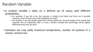
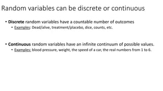
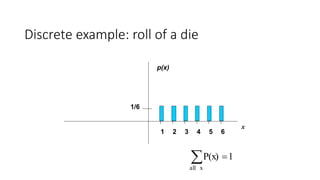
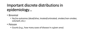
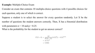
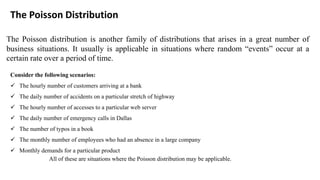
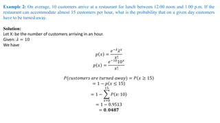
The document covers various probability distributions, including discrete (binomial, Poisson) and continuous (exponential, normal) distributions, detailing their definitions, examples, and calculations of probabilities and parameters such as mean and variance. It illustrates how random variables can be discrete or continuous, with specific applications in fields like epidemiology and statistics. Key examples are provided to demonstrate the binomial probability mass function and Poisson distribution, highlighting their applications in real-world scenarios.

1. Dr. Shivakumar B. N.
Assistant Professor
Department of Mathematics
CMR Institute of Technology
Bengaluru
Probability
Distribution

2. • Discrete: Binomial, Poisons, -mean and variance
(without proof) and problems.
• Continuous: Exponential, Normal -Mean and variance
(without proof) and problems.

3. Random Variable
•A random variable x takes on a defined set of values with different
probabilities.
• For example, if you roll a die, the outcome is random (not fixed) and there are 6 possible
outcomes, each of which occur with probability one-sixth.
• For example, if you poll people about their voting preferences, the percentage of the sample that
responds “Yes on Proposition 100” is a also a random variable (the percentage will be slightly
differently every time you poll).
• Examples are crop yield, maximum temperature, number of cyclones in a
season, rain/no rain.

4. Random variables can be discrete or continuous
• Discrete random variables have a countable number of outcomes
• Examples: Dead/alive, treatment/placebo, dice, counts, etc.
• Continuous random variables have an infinite continuum of possible values.
• Examples: blood pressure, weight, the speed of a car, the real numbers from 1 to 6.

5. Probability distributions
• If we measure a random variable many times, we can build up a
distribution of the values it can take.
• Imagine an underlying distribution of values which we would get if it was
possible to take more and more measurements under the same
conditions.
• This gives the probability distribution for the variable.

6. Probability functions
• A probability function maps the possible values of x against their respective
probabilities of occurrence, p(x)
• p(x) is a number from 0 to 1.0.
• The area under a probability function is always 1.

7. Discrete example: roll of a die
x
p(x)
1/6
1 4 5 6
2 3
 =
x
all
1
P(x)

8. Discrete probability distributions
• A discrete probability distribution associates a probability with each
value of a discrete random variable.
• Example 1. Random variable has two values Rain/No Rain. P(Rain) = 0.2, P(No
Rain) = 0.8 gives a probability distribution.
• Note that P(rain) + P(No Rain) = 1; P(X=0) + P(X=1) + P(X=2) + … +P(X=6) + …
P(X=10) = 1.

9. Continuous probability distributions
• Because continuous random variables can take all values in a range, it
is not possible to assign probabilities to individual values.
• Instead we have a continuous curve, called a probability density
function, which allows us to calculate the probability a value within
any interval.
• This probability is calculated as the area under the curve between the
values of interest. The total area under the curve must equal 1.

10. Important discrete distributions in
epidemiology…
• Binomial
• Yes/no outcomes (dead/alive, treated/untreated, smoker/non-smoker,
sick/well, etc.)
• Poisson
• Counts (e.g., how many cases of disease in a given area)

11. Binomial Distribution
Consider the following scenarios:
✓ The number of heads/tails in a sequence of coin flips.
✓ Vote counts for two different candidates in an election
✓ The number of male/female employees in a company
✓ The number of accounts that are in compliance or not in compliance with an accounting procedure
✓ The number of successful sales calls
✓ The number of defective products in a production run
All of these are situations where the binomial distribution may be applicable.

12. Binomial Probability-Mass Function
Let X be a binomial random variable. Then, its probability mass function is:
The values of n and p are called the parameters of the distribution.

13. Example: Multiple-Choice Exam
Consider an exam that contains 10 multiple-choice questions with 4 possible choices for
each question, only one of which is correct.
Suppose a student is to select the answer for every question randomly. Let X be the
number of questions the student answers correctly. Then, X has a binomial distribution
with parameters n = 10 and p = 0.25.
What is the probability for the student to get no answer correct?

14. What is the probability for the student to get two answers correct?

15. What is the probability for the student to fail the test (i.e., to have less than 6
correct answers)?

16. Example 2: 6 unbiased coins are tossed (a) Find the probability that the tosses result in (i)
heads only (ii) 3 heads (iii) 5 or more heads
Solution:
Given 𝑛 = 6; 𝑝 =
1
2
; 𝑞 = 1 − 𝑝 =
1
2
Let X: no. of heads obtained in 6 tosses.
Then
𝑝 𝑥 = 𝑛𝐶𝑥
𝑝𝑥𝑞𝑛−𝑥 𝑥 = 0,1,2, … 𝑛
→ 𝑝 𝑥 = 6𝐶𝑥
1
2
𝑥
1
2
6−𝑥
= 6𝐶𝑥
1
2
6
; 𝑥 = 0,1,2 … . . 6
(i) 𝑃 ℎ𝑒𝑎𝑑𝑠 𝑜𝑛𝑙𝑦 = 𝑃 𝑥 = 6
= 𝑝 6
= 6𝐶6
= 6𝐶6
1
2
6
= 𝟎. 𝟎𝟏𝟓𝟔

17. (ii) 𝑃 3 ℎ𝑒𝑎𝑑𝑠 = 𝑃 𝑋 = 3
= 𝑝 3
= 6𝐶3
1
2
6
= 𝟎. 𝟑𝟏𝟐𝟓
(iii) 𝑝 5 𝑜𝑟 𝑚𝑜𝑟𝑒 ℎ𝑒𝑎𝑑𝑠 = 𝑝 𝑥 ≥ 5
= 𝑝 5 + 𝑝 6
= 6𝐶5
1
2
6
+ 6𝐶6
1
2
6
= 𝟎. 𝟏𝟎𝟗𝟒

18. Mean and variance of binomial distribution
Mean, 𝐸 𝑋 = 𝑛𝑝
Variance, 𝑉𝑎𝑟 𝑋 = 𝑛𝑝𝑞
Note: For binomial distribution
Mean > Variance
Example 1: Find the mean and variance of a binomial experiment with 𝒏 = 𝟓 and 𝒑 = 𝟎. 𝟒
Solution:
Given 𝑛 = 5; 𝑝 = 0.4 ⟹ 𝑞 = 1 − 𝑝 = 0.6
Mean is given by
𝐸 𝑋 = 𝑛𝑝 = 5 0.4 = 𝟐

19. Example 2: If in a binomial distribution mean = 8 and variance = 1.6. Find 𝑷 𝑿 = 𝟐 and 𝑷 𝑿 = 𝟓 .
Solution:
Let the bino
mial variate be denote by X. Let n and p be the two parameters
Then, mean = 8 and variance = 1.6
i.e., np=8 and npq=1.6
Consider
𝑛𝑝𝑞
𝑛𝑝
=
1.6
8
⟹ 𝑞 = 0.2
⟹ 𝑝 = 1 − 𝑞 = 1 − 0.2 = 0.8
⟹ 𝑞 = 0.2 𝑎𝑛𝑑 𝑝 = 0.8
We know that, 𝑛𝑝 = 8
𝑛 0.8 = 8
𝑛 = 10
𝑝 𝑥 = 10𝐶𝑥
0.8 𝑥 0.2 10−𝑥 𝑥 = 0,1, … 10
(i) 𝑝 𝑥 = 2 = 𝑝 2
10𝐶2
0.8 2 0.2 8 = 𝟎. 𝟎𝟎𝟎𝟎𝟕
(i) (ii) 𝑝 𝑥 = 5 = 𝑝 5
10𝐶5 0.8 5 0.2 5 = 𝟎. 𝟎𝟐𝟔

20. The Poisson distribution is another family of distributions that arises in a great number of
business situations. It usually is applicable in situations where random “events” occur at a
certain rate over a period of time.
The Poisson Distribution
Consider the following scenarios:
✓ The hourly number of customers arriving at a bank
✓ The daily number of accidents on a particular stretch of highway
✓ The hourly number of accesses to a particular web server
✓ The daily number of emergency calls in Dallas
✓ The number of typos in a book
✓ The monthly number of employees who had an absence in a large company
✓ Monthly demands for a particular product
All of these are situations where the Poisson distribution may be applicable.

21. The Poisson Distribution
Definition: A discrete random variable X is said to follow Poisson
distribution if its probability mass function is given
𝑝 𝑥 =
𝑒−𝜆
𝜆𝑥
𝑥!
𝑥 = 0,1,2 …
𝜆 > 0
𝑒 = 2.718282 …

22. Example 1: The average number of telephone received by a receptionist of a large office between 9:30 a.m. and
9:45 a.m. is 5. Find the probability that on a randomly selected day 2 or more calls are received by the receptionist.
Solution:
Let X: be the number of telephone calls received between 9:30 and 9:45 a.m.
Given: 𝜆 = 5
We have
𝑝 𝑥 =
𝑒−𝜆
𝜆𝑥
𝑥!
𝑝 𝑥 =
𝑒−55𝑥
𝑥!
𝑃(2 𝑜𝑟 𝑚𝑜𝑟𝑒 𝑐𝑎𝑙𝑙𝑠) = 𝑃 𝑥 ≥ 2
= 1 − 𝑝 𝑥 < 2
= 1 − 𝑝 0 + 𝑝 1
= 1 −
𝑒−550
0!
+
𝑒−551
1!
= 1 − 0.0067 + 0.0067 5
= 𝟎. 𝟗𝟓𝟗𝟖

23. Example 2: On average, 10 customers arrive at a restaurant for lunch between 12.00 noon and 1.00 p.m. If the
restaurant can accommodate almost 15 customers per hour, what is the probability that on a given day customers
have to be turned away.
Solution:
Let X: be the number of customers arriving in an hour.
Given: 𝜆 = 10
We have
𝑝 𝑥 =
𝑒−𝜆𝜆𝑥
𝑥!
𝑝 𝑥 =
𝑒−10
10𝑥
𝑥!
𝑃(𝑐𝑢𝑠𝑡𝑜𝑚𝑒𝑟𝑠 𝑎𝑟𝑒 𝑡𝑢𝑟𝑛𝑒𝑑 𝑎𝑤𝑎𝑦) = 𝑃 𝑥 ≥ 15
= 1 − 𝑝 𝑥 ≤ 15
= 1 − ෍
𝑥=0
15
𝑃 𝑥: 10
= 1 − 0.9513
= 𝟎. 𝟎𝟒𝟖𝟕

24. Mean and Variance
𝐸 (𝑋) = 𝑉 (𝑋) = 𝜆

25. Example 1: For a Poisson variate, 3𝑝 2 = 𝑝 4 . Find the standard deviation of the distribution.
Solution:
Given: 3𝑝 2 = 𝑝 4
We have
𝑝 𝑥 =
𝑒−𝜆𝜆𝑥
𝑥!
3
𝑒−𝜆𝜆2
2!
=
𝑒−𝜆𝜆4
4!
𝜆2
= 36
𝜆 = 6
Hence the mean and variance of the distribution is 6 and
𝑆𝑡𝑎𝑛𝑑𝑎𝑟𝑑 𝐷𝑒𝑣𝑖𝑎𝑡𝑖𝑜𝑛 = 𝑣𝑎𝑟
= 6
= 𝟐. 𝟒𝟒𝟗

26. Exponential Distribution
Another useful continuous distribution is the exponential distribution, which has the
following probability density function:
Examples:
• The length of time between telephone calls
• The length of time between arrivals at a service station
• The life time of electronic components, i.e., an inter-failure time
𝒇 𝒙 = 𝜽𝒆−𝜽𝒙 𝒇𝒐𝒓 𝒙 ≥ 𝟎

27. Mean and Variance
𝐸 𝑥 =
1
𝜃
𝑉𝑎𝑟 𝑋 =
1
𝜃2

28. Example 1: Suppose that a system contains a certain type of component whose time in years to fall is given by T. By
experience, it is known that the random variable T follows an exponential distribution with mean time to failure = 5. Find the
probability that the system is functioning at the end of 8 years.
Solution:
Let T be time in years to fail
Given 𝐸 𝑇 = 5
1
𝜃
= 5
𝜃 = 0.2
𝑃 𝑠𝑦𝑠𝑡𝑒𝑚 𝑖𝑠 𝑓𝑢𝑛𝑐𝑡𝑖𝑜𝑛 𝑎𝑡 𝑒𝑛𝑑 𝑜𝑓 8 𝑦𝑒𝑎𝑟𝑠 = 𝑃 𝑇 > 8
We know that
𝑃 𝑇 ≤ 𝑡 = 1 − 𝑒−𝜃𝑡
𝑃 𝑇 > 𝑡 = 𝑒−𝜃𝑡
𝑃 𝑇 > 8 = 𝑒−0.2∗8
= 𝑒−1.6
𝟎. 𝟐𝟎𝟏𝟖

29. Normal Probability Distributions

30. • This is the most popular distribution for
continuous random variables
• First described de Moivre in 1733
• Elaborated in 1812 by Laplace
• Describes some natural phenomena
• More importantly, describes sampling
characteristics of totals and means

31. … we can easily
determine the Area in
tails
95%
Because the Normal
curve is symmetrical
and the total AUC is
exactly 1…
Symmetry in the Tails

33. Example: x is a normal variate with mean 50 and standard deviation 4. Find the probability that a value taken by x is
(i) Less than 54
(ii) Less than 50
(iii) Between 42 and 48
(iv) Between 52 and 56
(v) Greater than 58
(vi) Greater than 48
Solution:
𝑍 =
𝑋 − 𝜇
𝜎
=
𝑋 − 50
4
(i) 𝑍 =
𝑋−50
4
=
54−50
4
= 𝐴𝑟𝑒𝑎 𝑓𝑟𝑜𝑚 0 𝑡𝑜 1 = 𝟎. 𝟖𝟒𝟏𝟑
(ii) 𝑍 =
𝑋−50
4
=
50−50
4
=0=0.5