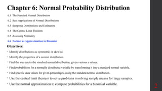
Elementary Statistics
Chapter 6:
Normal Probability
Distribution
6.6 Normal as
Approximation to
Binomial
1
Chapter 6: Normal Probability Distribution
6.1 The Standard Normal Distribution
6.2 Real Applications of Normal Distributions
6.3 Sampling Distributions and Estimators
6.4 The Central Limit Theorem
6.5 Assessing Normality
6.6 Normal as Approximation to Binomial
2
Objectives:
• Identify distributions as symmetric or skewed.
• Identify the properties of a normal distribution.
• Find the area under the standard normal distribution, given various z values.
• Find probabilities for a normally distributed variable by transforming it into a standard normal variable.
• Find specific data values for given percentages, using the standard normal distribution.
• Use the central limit theorem to solve problems involving sample means for large samples.
• Use the normal approximation to compute probabilities for a binomial variable.
Key Concept:
Use a normal distribution as an approximation to the binomial probability distribution: BD:
n & p⇾ q = 1 − p
If the conditions of np ≥ 5 and nq ≥ 5 (approximation is better if np ≥ 10 and nq ≥ 10) are both
satisfied, then probabilities from a binomial probability distribution can be approximated reasonably
well by using a normal distribution having these parameters: 𝜇 = 𝑛𝑝 & 𝜎 = 𝑛𝑝𝑞
The binomial probability distribution is discrete (with whole numbers for the random variable x), but
the normal approximation is continuous. To compensate, we use a “continuity correction” with a
whole number x represented by the interval from x − 0.5 to x + 0.5.
Recall: A binomial probability distribution has
(1) a fixed number of trials;
(2) trials that are independent;
(3) trials that are each classified into two categories commonly referred to as success and failure;
and
(4) trials with the property that the probability of success remains constant.
6.6 Normal as Approximation to Binomial
3
Notation
n = the fixed number of trials
x = the specific number of successes in n trials
p = probability of success in one of the n trials
q = probability of failure in one of the n trials (so q = 1 − p)
Rationale for Using a Normal Approximation:
Recall: The sampling distribution of a sample proportion tends to approximate a normal
distribution.
Check the following probability histogram for the binomial distribution:
n = 580 & p = 0.25.
(In one of Mendel’s famous hybridization experiments, he expected 25% of his 580 peas to be
yellow, but he got 152 yellow peas, for a rate of 26.2%.) The bell-shape of this graph suggests
that we can use a normal distribution to approximate the binomial distribution.
6.6 Normal as Approximation to Binomial
4
Requirements
1. The sample is a simple random sample of size n from a population in which the proportion of
successes is p, or the sample is the result of conducting n independent trials of a binomial
experiment in which the probability of success is p.
2. np ≥ 5 and nq ≥ 5. (approximation is better if np ≥ 10 and nq ≥ 10)
Normal Approximation
If the above requirements are satisfied, then the probability distribution of the random variable x can be
approximated by a normal distribution with these parameters: 𝜇 = 𝑛𝑝 & 𝜎 = 𝑛𝑝𝑞
Continuity Correction
When using the normal approximation, adjust the discrete whole number x by using a continuity correction so that any
individual value x is represented in the normal distribution by the interval from x − 0.5 to x + 0.5.
Procedure:
1. Check the requirements that np ≥ 5 and nq ≥ 5.
2. Find 𝜇 = 𝑛𝑝 & 𝜎 = 𝑛𝑝𝑞
3. Identify the discrete whole number x that is relevant to the binomial probability problem being considered, and
represent that value by the region bounded by x − 0.5 and x + 0.5.
4. Graph the normal distribution and shade the desired area bounded by x − 0.5 or x + 0.5 as appropriate.
6.6 Normal as Approximation to Binomial
5
6.6 Normal as Approximation to Binomial
The Normal Approximation to the Binomial Distribution
Binomial
When finding:
P(X = a)
P(X  a)
P(X > a)
P(X  a)
P(X < a)
Normal
Use:
P(a – 0.5 < X < a + 0.5)
P(X > a – 0.5)
P(X > a + 0.5)
P(X < a + 0.5)
P(X < a – 0.5)
For all cases, 𝜇 = 𝑛𝑝, 𝜎 = 𝑛𝑝𝑞, 𝑛𝑝 ≥ 5, 𝑛𝑞 ≥ 5
6
7
Assume that 6% of American drivers text while driving. If 300
drivers are selected at random, find the probability that exactly
25 say they text while driving. (Use Normal approximation)
Example 1
Given: Binomial Distribution(BD), n = 300 & p = 0.06
np = (300)(0.06) = 18 ≥ 5 and nq = (300)(0.94) = 282 ≥ 5
𝜇 = 𝑛𝑝 = 300(0.06) = 18
𝜎 = 𝑛𝑝𝑞 = 300 0.06 0.94 = 4.1134
𝐵𝐷: 𝑃(𝑥 = 25) = 𝑁𝐷: 𝑃(24.5 < 𝑥 < 25.5) =
𝑧 =
24.5 − 18
4.11
= 1.58,
𝑧 =
25.5 − 18
4.11
= 1.82
0.9656 – 0.9429 = 0.0227
𝑆𝑁𝐷: 𝑃(1.58 < 𝑧 < 1.82) =
𝜇 = 𝑛𝑝, 𝜎 = 𝑛𝑝𝑞, 𝑛𝑝 ≥ 5, 𝑛𝑞 ≥ 5 𝑧 =
𝑥 − 𝜇
𝜎
8
Suppose 10% of the members of a
handball league are left-handed. If 200
handball league members are selected
at random, find the probability that
a. 10 or more will be left-handed.
b. At most 15 will be left-handed.
Example 2
Given: Binomial Distribution(BD), n = 200 & p = 0.1
np = (200)(0.10) = 20 and nq = (200)(0.90) = 180 ⇾
np ≥ 5 & nq ≥ 5
𝜇 = 𝑛𝑝 = 200(0.1) = 20
𝜎 = 𝑛𝑝𝑞 = 200 0.10 0.90 = 4.24
𝐵𝐷: 𝑃(𝑥 ≥ 10) = 𝑁𝐷: 𝑃(𝑥 > 9.5) = 𝑧 =
9.5 − 20
4.24
= −2.48
𝑆𝑁𝐷: 𝑃(𝑧 > −2.48) = 1.0000 – 0.0066 = 0.9934
𝜇 = 𝑛𝑝, 𝜎 = 𝑛𝑝𝑞, 𝑛𝑝 ≥ 5, 𝑛𝑞 ≥ 5 𝑧 =
𝑥 − 𝜇
𝜎
𝐵𝐷: 𝑃(𝑥 ≤ 15) = 𝑁𝐷: 𝑃(𝑥 < 15.5) = 𝑆𝑁𝐷: 𝑃(𝑧 < −1.06) =
0.1446
𝑧 =
15.5 − 20
4.24
= −1.06
9
In one of Mendel’s famous hybridization experiments, he expected that among 580
offspring peas, 145 of them (or 25%) would be yellow, but he actually got 152 yellow
peas. Assuming that Mendel’s rate of 25% is correct, find
a. P(exactly 152 yellow peas).
b. find the probability of getting 152 or more yellow peas by random chance. That is,
given n = 580 and p = 0.25, find P(at least 152 yellow peas).
Example 3
Given: Binomial Distribution(BD), n = 580 & p = 0.25
np = (580)(0.25) = 145 & nq = (580)(0.75) = 435 ⇾ np ≥ 5 & nq ≥ 5
𝜇 = 𝑛𝑝 = 580(0.25) = 145
𝜎 = 𝑛𝑝𝑞 = 580(0.25)(0.75) = 10.4283
𝜇 = 𝑛𝑝, 𝜎 = 𝑛𝑝𝑞, 𝑛𝑝 ≥ 5, 𝑛𝑞 ≥ 5
𝐵𝐷: 𝑃(𝑥 = 152) =
𝑁𝐷: 𝑃(151.5 < 𝑥 < 152.5)
𝑧 =
𝑥 − 𝜇
𝜎
𝑧 =
𝑥 − 𝜇
𝜎
=
151.5 − 145
10.4283
= 0.62
𝑧 =
𝑥 − 𝜇
𝜎
=
152.5 − 145
10.4283
= 0.72
0.7642 − 0.7324 = 0.0318
𝑆𝑁𝐷: 𝑃(0.62 < 𝑧 < 0.72) =
10
b. P(at least 152 yellow peas)
𝐵𝐷: 𝑃(𝑥 ≥ 152) =
𝑁𝐷: 𝑃(𝑥 > 151.5) =
𝑆𝑁𝐷: 𝑃(𝑧 > 0.62) = 1 − 0.7324 = 0.2676
Technology for Binomial
Probabilities (Statdisk)

Normal as Approximation to Binomial

  • 1.
    Elementary Statistics Chapter 6: NormalProbability Distribution 6.6 Normal as Approximation to Binomial 1
  • 2.
    Chapter 6: NormalProbability Distribution 6.1 The Standard Normal Distribution 6.2 Real Applications of Normal Distributions 6.3 Sampling Distributions and Estimators 6.4 The Central Limit Theorem 6.5 Assessing Normality 6.6 Normal as Approximation to Binomial 2 Objectives: • Identify distributions as symmetric or skewed. • Identify the properties of a normal distribution. • Find the area under the standard normal distribution, given various z values. • Find probabilities for a normally distributed variable by transforming it into a standard normal variable. • Find specific data values for given percentages, using the standard normal distribution. • Use the central limit theorem to solve problems involving sample means for large samples. • Use the normal approximation to compute probabilities for a binomial variable.
  • 3.
    Key Concept: Use anormal distribution as an approximation to the binomial probability distribution: BD: n & p⇾ q = 1 − p If the conditions of np ≥ 5 and nq ≥ 5 (approximation is better if np ≥ 10 and nq ≥ 10) are both satisfied, then probabilities from a binomial probability distribution can be approximated reasonably well by using a normal distribution having these parameters: 𝜇 = 𝑛𝑝 & 𝜎 = 𝑛𝑝𝑞 The binomial probability distribution is discrete (with whole numbers for the random variable x), but the normal approximation is continuous. To compensate, we use a “continuity correction” with a whole number x represented by the interval from x − 0.5 to x + 0.5. Recall: A binomial probability distribution has (1) a fixed number of trials; (2) trials that are independent; (3) trials that are each classified into two categories commonly referred to as success and failure; and (4) trials with the property that the probability of success remains constant. 6.6 Normal as Approximation to Binomial 3
  • 4.
    Notation n = thefixed number of trials x = the specific number of successes in n trials p = probability of success in one of the n trials q = probability of failure in one of the n trials (so q = 1 − p) Rationale for Using a Normal Approximation: Recall: The sampling distribution of a sample proportion tends to approximate a normal distribution. Check the following probability histogram for the binomial distribution: n = 580 & p = 0.25. (In one of Mendel’s famous hybridization experiments, he expected 25% of his 580 peas to be yellow, but he got 152 yellow peas, for a rate of 26.2%.) The bell-shape of this graph suggests that we can use a normal distribution to approximate the binomial distribution. 6.6 Normal as Approximation to Binomial 4
  • 5.
    Requirements 1. The sampleis a simple random sample of size n from a population in which the proportion of successes is p, or the sample is the result of conducting n independent trials of a binomial experiment in which the probability of success is p. 2. np ≥ 5 and nq ≥ 5. (approximation is better if np ≥ 10 and nq ≥ 10) Normal Approximation If the above requirements are satisfied, then the probability distribution of the random variable x can be approximated by a normal distribution with these parameters: 𝜇 = 𝑛𝑝 & 𝜎 = 𝑛𝑝𝑞 Continuity Correction When using the normal approximation, adjust the discrete whole number x by using a continuity correction so that any individual value x is represented in the normal distribution by the interval from x − 0.5 to x + 0.5. Procedure: 1. Check the requirements that np ≥ 5 and nq ≥ 5. 2. Find 𝜇 = 𝑛𝑝 & 𝜎 = 𝑛𝑝𝑞 3. Identify the discrete whole number x that is relevant to the binomial probability problem being considered, and represent that value by the region bounded by x − 0.5 and x + 0.5. 4. Graph the normal distribution and shade the desired area bounded by x − 0.5 or x + 0.5 as appropriate. 6.6 Normal as Approximation to Binomial 5
  • 6.
    6.6 Normal asApproximation to Binomial The Normal Approximation to the Binomial Distribution Binomial When finding: P(X = a) P(X  a) P(X > a) P(X  a) P(X < a) Normal Use: P(a – 0.5 < X < a + 0.5) P(X > a – 0.5) P(X > a + 0.5) P(X < a + 0.5) P(X < a – 0.5) For all cases, 𝜇 = 𝑛𝑝, 𝜎 = 𝑛𝑝𝑞, 𝑛𝑝 ≥ 5, 𝑛𝑞 ≥ 5 6
  • 7.
    7 Assume that 6%of American drivers text while driving. If 300 drivers are selected at random, find the probability that exactly 25 say they text while driving. (Use Normal approximation) Example 1 Given: Binomial Distribution(BD), n = 300 & p = 0.06 np = (300)(0.06) = 18 ≥ 5 and nq = (300)(0.94) = 282 ≥ 5 𝜇 = 𝑛𝑝 = 300(0.06) = 18 𝜎 = 𝑛𝑝𝑞 = 300 0.06 0.94 = 4.1134 𝐵𝐷: 𝑃(𝑥 = 25) = 𝑁𝐷: 𝑃(24.5 < 𝑥 < 25.5) = 𝑧 = 24.5 − 18 4.11 = 1.58, 𝑧 = 25.5 − 18 4.11 = 1.82 0.9656 – 0.9429 = 0.0227 𝑆𝑁𝐷: 𝑃(1.58 < 𝑧 < 1.82) = 𝜇 = 𝑛𝑝, 𝜎 = 𝑛𝑝𝑞, 𝑛𝑝 ≥ 5, 𝑛𝑞 ≥ 5 𝑧 = 𝑥 − 𝜇 𝜎
  • 8.
    8 Suppose 10% ofthe members of a handball league are left-handed. If 200 handball league members are selected at random, find the probability that a. 10 or more will be left-handed. b. At most 15 will be left-handed. Example 2 Given: Binomial Distribution(BD), n = 200 & p = 0.1 np = (200)(0.10) = 20 and nq = (200)(0.90) = 180 ⇾ np ≥ 5 & nq ≥ 5 𝜇 = 𝑛𝑝 = 200(0.1) = 20 𝜎 = 𝑛𝑝𝑞 = 200 0.10 0.90 = 4.24 𝐵𝐷: 𝑃(𝑥 ≥ 10) = 𝑁𝐷: 𝑃(𝑥 > 9.5) = 𝑧 = 9.5 − 20 4.24 = −2.48 𝑆𝑁𝐷: 𝑃(𝑧 > −2.48) = 1.0000 – 0.0066 = 0.9934 𝜇 = 𝑛𝑝, 𝜎 = 𝑛𝑝𝑞, 𝑛𝑝 ≥ 5, 𝑛𝑞 ≥ 5 𝑧 = 𝑥 − 𝜇 𝜎 𝐵𝐷: 𝑃(𝑥 ≤ 15) = 𝑁𝐷: 𝑃(𝑥 < 15.5) = 𝑆𝑁𝐷: 𝑃(𝑧 < −1.06) = 0.1446 𝑧 = 15.5 − 20 4.24 = −1.06
  • 9.
    9 In one ofMendel’s famous hybridization experiments, he expected that among 580 offspring peas, 145 of them (or 25%) would be yellow, but he actually got 152 yellow peas. Assuming that Mendel’s rate of 25% is correct, find a. P(exactly 152 yellow peas). b. find the probability of getting 152 or more yellow peas by random chance. That is, given n = 580 and p = 0.25, find P(at least 152 yellow peas). Example 3 Given: Binomial Distribution(BD), n = 580 & p = 0.25 np = (580)(0.25) = 145 & nq = (580)(0.75) = 435 ⇾ np ≥ 5 & nq ≥ 5 𝜇 = 𝑛𝑝 = 580(0.25) = 145 𝜎 = 𝑛𝑝𝑞 = 580(0.25)(0.75) = 10.4283 𝜇 = 𝑛𝑝, 𝜎 = 𝑛𝑝𝑞, 𝑛𝑝 ≥ 5, 𝑛𝑞 ≥ 5 𝐵𝐷: 𝑃(𝑥 = 152) = 𝑁𝐷: 𝑃(151.5 < 𝑥 < 152.5) 𝑧 = 𝑥 − 𝜇 𝜎 𝑧 = 𝑥 − 𝜇 𝜎 = 151.5 − 145 10.4283 = 0.62 𝑧 = 𝑥 − 𝜇 𝜎 = 152.5 − 145 10.4283 = 0.72 0.7642 − 0.7324 = 0.0318 𝑆𝑁𝐷: 𝑃(0.62 < 𝑧 < 0.72) =
  • 10.
    10 b. P(at least152 yellow peas) 𝐵𝐷: 𝑃(𝑥 ≥ 152) = 𝑁𝐷: 𝑃(𝑥 > 151.5) = 𝑆𝑁𝐷: 𝑃(𝑧 > 0.62) = 1 − 0.7324 = 0.2676 Technology for Binomial Probabilities (Statdisk)