Downloaded 11 times

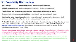
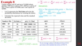
![Parameters of a Probability Distribution
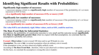
Remember that with a probability
distribution, we have a description of a
population instead of a sample, so the
values of the mean, standard deviation,
and variance are parameters, not
statistics.
The mean, variance, and standard
deviation of a discrete probability
distribution can be found with the
following formulas:
Mean (Expected Value), Variance &
Standard Deviation of D.R.V x:
Mean (the expected value) of
occurrence per repetition (it represents
the average value of the outcome):
10
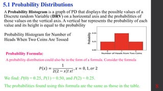
5.1 Probability Distributions
μ = 𝐸 𝑥 = 𝑥𝑝(𝑥)
𝜇 = 𝐸(𝑥) = 𝑥𝑝(𝑥)
𝜎 = (𝑥 − 𝜇)2𝑝(𝑥) = 𝑥2𝑝(𝑥) − 𝜇2 ,
Pr 𝑜 𝑜𝑓
(𝑥 − 𝜇)2𝑝(𝑥) = (𝑥2 − 2𝜇𝑥 + 𝜇2)𝑝(𝑥)
= 𝑥2𝑝(𝑥) − 𝜇[2 𝑥𝑝(𝑥) − 𝜇 𝑝 (𝑥)]
= 𝑥2
𝑝(𝑥) − 𝜇[2𝜇 − 𝜇 • 1] = 𝑥2
𝑝(𝑥) − 𝜇2
Variance:
𝜎2
= 𝑥2
⋅ 𝑃(𝑥) − 𝜇2](https://image.slidesharecdn.com/sec5-210709194220/85/Probability-Distribution-10-320.jpg)
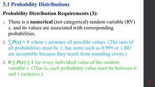
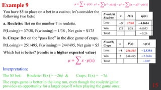
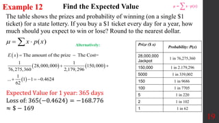
![Example 5
Given a probability distribution for rolling a single die, find
a. the mean.
b. the variance and standard deviation.
11
Probability Distributions
𝜇 = 𝑥 ⋅ 𝑝(𝑥)
= 1 ⋅
1
6
+ 2 ⋅
1
6
+ 3 ⋅
1
6
+ 4 ⋅
1
6
+ 5 ⋅
1
6
+ 6 ⋅
1
6
=
21
6
= 3.5
Outcome x P(x)
1 1/6
2 1/6
3 1/6
4 1/6
5 1/6
6 1/6
= [12
⋅
1
6
+ 22
⋅
1
6
+ 32
⋅
1
6
+ 42
⋅
1
6
+52
⋅
1
6
+ 62
⋅
1
6
] − 3.5 2
𝜎2 = 2.91667
𝜎 = 1.70783
𝜎2
= 𝑥2
⋅ 𝑝(𝑥) − 𝜇2
= (𝑥 − 𝜇)2
⋅ 𝑝(𝑥)
𝜇 = 𝐸(𝑥) = 𝑥𝑝(𝑥)
𝜎 = (𝑥 − 𝜇)2𝑝(𝑥)
= 𝑥2𝑝(𝑥) − 𝜇2
𝜎2 = 𝑥2 ⋅ 𝑝(𝑥) − 𝜇2 =
Interpretation: If we were to collect data on
rolling a single die many times, we expect to
get a mean of 3.5 and SD of 1.708.](https://image.slidesharecdn.com/sec5-210709194220/85/Probability-Distribution-11-320.jpg)
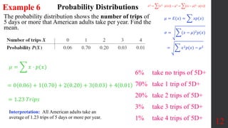
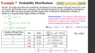

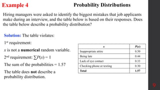
Chapter 5 covers discrete probability distributions, focusing on constructing distributions for random variables and calculating their mean, variance, and standard deviation. It explains the significance of probability distributions, including requirements and parameters, and illustrates various examples such as rolling dice and lottery probabilities. The chapter emphasizes understanding expected values and identifying significant outcomes in probability experiments.