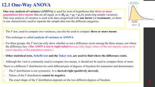
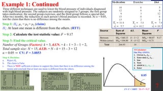
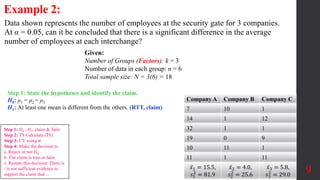
Chapter 12 discusses Analysis of Variance (ANOVA), specifically focusing on one-way and two-way ANOVA techniques to determine significant differences among three or more means. It explains the use of the F test for hypothesis testing, assumptions for the ANOVA, and how to calculate between-group and within-group variances. The chapter also includes examples illustrating how to apply the ANOVA method and interpret results, with supporting resources for further learning.

1. Elementary Statistics
Chapter 12:
Analysis of Variance
12.1 One-Way ANOVA
1

2. Chapter 12: Analysis of Variance
12.1 One-Way ANOVA
12.2 Two-Way ANOVA
2
Objectives:
Use the ANOVA technique to determine if there is a significant
difference among three or more means.
Good lecture Videos to watch: ANOVA
Concept: https://www.youtube.com/watch?v=ITf4vHhyGpc
Hand Calculation: https://www.youtube.com/watch?v=WUjsSB7E-ko
Visual Explanation: https://www.youtube.com/watch?v=JgMFhKi6f6Y
YouTube: https://www.youtube.com/watch?v=YbX-JUqD1so
Tukey Website + ANOVA:
https://astatsa.com/OneWay_Anova_with_TukeyHSD/
One-Way (Single Factor) ANOVA + Tukey
1. Get rid of the check mark
2. Choose the value of K (Number of treatment columns)
3. Proceed to enter your treatment columns
4. Enter Data
5. Calculate ANOVA with Tukey, Scheffe, Bonferroni & Holm
6. All is Ready

3. 3
12.1 One-Way ANOVA
One-way analysis of variance (ANOVA) is used for tests of hypotheses that three or more
populations have means that are all equal, as in H0: µ1 = µ2 = µ3 by analyzing sample variances.
One-way analysis of variance is used with data categorized with one factor (or treatment), so there
is one characteristic used to separate the sample data into the different categories.
• The F test, used to compare two variances, can also be used to compare three or more means.
• This technique is called analysis of variance or ANOVA.
• For three groups, the F test can only show whether or not a difference exists among the three means, not where
the difference lies. (The ANOVA test is right-tailed because only large values of the test statistic cause us to
reject equality of the population means.)
• Other statistical tests, Scheffé test and the Tukey test, are used to find where the difference exists.
• Although the t test is commonly used to compare two means, it should not be used to compare three or more.
There is a different F distribution for each different pair of degrees of freedom for numerator and denominator.
1. The F distribution is not symmetric. It is skewed right (positively skewed).
2. Values of the F distribution cannot be negative.
3. The exact shape of the F distribution depends on the two different degrees of freedom.

4. 4
12.1 One-Way ANOVA
In the F test, two different estimates of the population variance are made.
The first estimate is called the between-group variance, and it involves finding the variance of the means.
The second estimate, the within-group variance, is made by computing the variance using all the data
and is not affected by differences in the means.
If there is no difference in the means, the between-group variance will be approximately equal to the
within-group variance, and the F test value will be close to 1; do not reject null hypothesis.
However, when the means differ significantly, the between-group variance will be much larger than
the within-group variance; the F test will be significantly greater than 1; reject null hypothesis.
The following assumptions apply when using the F test to compare three or more means.
1. The populations from which the samples were obtained must be normally or approximately
normally distributed.
2. The samples must be independent of each other.
3. The populations have the same variance σ² (or standard deviation σ).
4. The samples are simple random samples of quantitative data.
5. The different samples are from populations that are categorized in only one way.
Step 1: H0 , H1, claim & Tails
Step 2: TS Calculate (TS)
Step 3: CV using α
Step 4: Make the decision to
a. Reject or not H0
b. The claim is true or false
c. Restate this decision: There is
/ is not sufficient evidence to
support the claim that…

5. 5
Example 1:
Three different techniques are used to lower the blood pressure of
individuals diagnosed with high blood pressure. The subjects are
randomly assigned to 3 groups; the first group takes medication, the
second group exercises, and the third group follows a special diet. After
two months, the reduction in each person’s blood pressure is recorded.
At α = 0.05, test the claim that there is no difference among the means.
Step 1: State the hypotheses and identify the claim.
H0: μ1 = μ2 = μ3 (claim)
H1: At least one mean is different from the others. (RTT)
Given:
Number of Groups (Factors): k = 3
Number of data in each group: n = 5
Total sample size: N = 3(5) = 15
Sum of Squares: SST = SSW + SSB
The total sum of squares: Find the squared distances
from the Grand Mean. (If we took the average, we
would have a variance.)
The within-group or within-cell sum of squares comes
from the distance of the observations to the cell
means. This indicates error.
The between-cells or between-groups sum of squares
tells of the distance of the cell means from the grand
mean. This indicates treatment (the column) effects.
𝑆𝑆𝑡𝑜𝑡 = 𝑆𝑆𝐵 + 𝑆𝑆𝑊 = (𝑋𝑖 − 𝑋𝐺)2
𝑆𝑆𝑊 = (𝑋𝑖 − 𝑋𝐴)2
= (𝑋1 − 𝑋1)2
+ (𝑋2 − 𝑋2)2
+ (𝑋3 − 𝑋3)2
+. . .
𝑆𝑆𝐵 = 𝑁𝐴(𝑋𝐴 − 𝑋𝐺)2
𝑂𝑅 = 𝑆𝑆𝑡𝑜𝑡 − 𝑆𝑆𝑊
𝑋𝑖: Each piece of Data,
𝑋𝐺: The Grand Mean, taken over all observations.
𝑋𝐴: The mean of any level of a treatment.

6. 6
Example 1: Continued
Step 2: Calculate the test statistic value.
a. Find the mean and variance of each sample (Given Table).
𝑥𝐺𝑀 =
𝑥
𝑁
=
10 + 12 + 9 + 15 + 13 + 6 + ⋯ + 4
15
𝑀𝑆𝐵 𝑂𝑅 𝑠𝐵
2
=
𝑆𝑆𝐵
𝑘 − 1
=
𝑛𝑖 𝑋𝑖 − 𝑋𝐺𝑀
2
𝑘 − 1
=
5 11.8 − 7.73 2
+ 5 3.8 − 7.73 2
+ 5 7.6 − 7.73 2
3 − 1
𝑀𝑆𝑤 𝑂𝑅 𝑠𝑊
2
𝑂𝑅 𝑠𝑝
2
=
𝑆𝑆𝑤
𝑁 − 𝑘
=
𝑛𝑖 − 1 𝑠𝑖
2
𝑛𝑖 − 1
=
4 5.7 + 4 10.2 + 4 10.3
4 + 4 + 4
𝐹 =
MS𝐵
MS𝑊
=
𝑠𝐵
2
𝑠𝑊
2
=
116
15
= 7.73
=
160.13
2
= 80.07
=
104.80
12
= 8.73
Given the means of each group: 11.8, 3.8 & 7.6
Calculate their weighted average and variance:
𝑏. . 𝑥𝐺𝑀 =
𝑥𝑖
𝑘
=
11.8 + 3.8 + 7.6
3
= 7.73
𝑐. 𝑠𝑥
2
=
𝑥𝑖 − 𝑥𝐺𝑀
2
𝑘 − 1
=
11.8 − 7.73 2
+ 3.8 − 7.73 2
+ 7.6 − 7.76 2
3 − 1
≈ 16.018
𝑆𝐵 = 𝜎𝑥 =
𝜎
𝑛
→ 𝐸𝑠𝑡𝑖𝑚𝑎𝑡𝑒: 𝜎2
= 𝑛𝑠𝑥
2
→ 𝑀𝑆𝐵 𝑂𝑅 𝑠𝐵
2
= 𝑛𝑠𝑥
2
= 5(16.018) = 80.09
b. Find the Grand Mean, the mean of all values in the samples.
c. Find the Between-group variance (Mean Square, MSB.)
d. Find the Within-group variance (Error)(Mean
of sample variances, or mean square, MSW)
e. Calculate the F value.
𝑑. 𝑠𝑊
2
𝑂𝑅 𝑠𝑝
2
=
𝑆1
2
+ 𝑆2
2
+ 𝑆3
2
3
=
5.7 + 10.2 + 10.3
3
= 8.733
Source Sum of
Squares
d.f. Mean
Squares
F
Between
Within (error)
SSB =160.13
SSW =104.80
k – 1= 2
N – k=12
MSB = 80.07
MSW = 8.73
9.17
Total 264.93 14
=
80.07
8.73
= 9.17

7. 7
Three different techniques are used to lower the blood pressure of individuals diagnosed
with high blood pressure. The subjects are randomly assigned to 3 groups; the first group
takes medication, the second group exercises, and the third group follows a special diet.
After two months, the reduction in each person’s blood pressure is recorded. At α = 0.05,
test the claim that there is no difference among the means.
Step 3: Find the critical value.
Number of Groups (Factors): k = 3, d.f.N. = k – 1 = 3 – 1 = 2,
Total sample size: N = 15, d.f.D. = N – k = 15 – 3 = 12
α = 0.05 → CV: 𝑭 = 3.8853
Step 4: Decision:
a. Reject H0
b. The claim is False
c. There is NOT sufficient evidence to support the claim that there is no difference among the
means and conclude that at least one mean is different from the others.
Step 1: H0: μ1 = μ2 = μ3 (claim)
H1: At least one mean is different from the others. (RTT)
Step 2: Calculate the test statistic value: 𝐹 = 9.17
Example 1: Continued
CV: F = 3.8853 TS: 𝑭 = 9.17
0.05
Source Sum of
Squares
d.f. Mean
Squares
F
Between
Within (error)
SSB =160.13
SSW =104.80
k – 1= 2
N – k=12
MSB = 80.07
MSW = 8.73
9.17
Total 264.93 14
TI Calculator:
One Way ANOVA
1. ClrList 𝑳𝟏, 𝑳𝟐, …
2. Enter data 𝑳𝟏, 𝑳𝟐, . .
3. Stat
4. Tests
5. 𝑨𝑵𝑶𝑽𝑨 (𝑳𝟏, 𝑳𝟐 , . . )
6. Enter

8. 8
The between-group variance is sometimes
called the mean square, MSB.
• The numerator of the formula to
compute MSB is called the sum of
squares between groups, SSB.
• The within-group variance is sometimes
called the mean square, MSW.
• The numerator of the formula to
compute MSW is called the sum of
squares within groups, SSW.
Source Sum of
Squares
d.f. Mean
Squares = SS /df
𝑭 =
𝑴𝑺𝑩
𝑴𝑺𝒘
Squares = SS /df SSB =160.13
SSW =104.80
k – 1= 2
N – k=12
MSB = SSB / 2 = 80.07
MSW = SSW / 12 = 8.73
𝟖𝟎. 𝟎𝟕
𝟖. 𝟕𝟑
= 𝟗. 𝟏𝟕
Total SST = 264.93 14
12.1 One-Way ANOVA Summary Table
The Grand Mean,
taken over all
observations:
𝑥𝐺𝑀 =
𝑥
𝑁
=
𝑥𝑖
𝑘
Number of Groups (Factors): k
Number of data in each group: 𝒏𝟏, 𝒏𝟐,…
Total sample size: 𝑵 = 𝒏𝟏 + 𝒏𝟐 + ⋯
Each piece of data: 𝑿𝒊
Each Group (treatment) Mean: 𝒙𝒊
Between-group variance (Mean Square, MSB.)
𝑀𝑆𝐵 𝑂𝑅 𝑠𝐵
2
=
𝑆𝑆𝐵
𝑘 − 1
=
𝑛𝑖 𝑋𝑖 − 𝑋𝐺𝑀
2
𝑘 − 1
→ 𝑀𝑆𝐵 𝑂𝑅 𝑠𝐵
2
= 𝑛𝑠𝑥
2
, if same number of data in each
category (n times the variance for sample means)
Within-group variance (Error)(Mean of sample variances, or mean
square, MSW): 𝑀𝑆𝑤 𝑂𝑅 𝑠𝑊
2
𝑂𝑅 𝑠𝑝
2
=
𝑆𝑆𝑤
𝑁−𝑘
=
𝑛𝑖−1 𝑠𝑖
2
𝑛𝑖−1
𝑂𝑅 𝑠𝑝
2
=
𝑆1
2+𝑆2
2+𝑆3
2+⋯
𝑘
, if same number of data in each category

9. 9
Data shown represents the number of employees at the security gate for 3 companies.
At α = 0.05, can it be concluded that there is a significant difference in the average
number of employees at each interchange?
Example 2:
Company A Company B Company C
7 10 1
14 1 12
32 1 1
19 0 9
10 11 1
11 1 11
𝑥1 = 15.5,
𝑠1
2
= 81.9
𝑥2 = 4.0,
𝑠2
2
= 25.6
𝑥3 = 5.8,
𝑠3
2
= 29.0
Step 1: State the hypotheses and identify the claim.
H0: μ1 = μ2 = μ3
H1: At least one mean is different from the others. (RTT, claim)
Step 1: H0 , H1, claim & Tails
Step 2: TS Calculate (TS)
Step 3: CV using α
Step 4: Make the decision to
a. Reject or not H0
b. The claim is true or false
c. Restate this decision: There is
/ is not sufficient evidence to
support the claim that…
Given:
Number of Groups (Factors): k = 3
Number of data in each group: n = 6
Total sample size: N = 3(6) = 18

10. 10
Example 2: Continued
Step 2: Calculate the test statistic value.
a. Find the mean and variance of each sample (Given).
𝑥𝐺𝑀 =
𝑥
𝑁
=
7 + 14 + 32 + ⋯ + 11
18
𝑠𝐵
2
=
𝑛𝑖 𝑋𝑖 − 𝑋𝐺𝑀
2
𝑘 − 1
=
6 15.5 − 8.4333 2 + 6 4 − 8.4333 2 + 6 5.8 − 8.4333 2
3 − 1
𝑠𝑊
2
𝑂𝑅 𝑠𝑝
2 =
𝑛𝑖 − 1 𝑠𝑖
2
𝑛𝑖 − 1
=
5 81.9 + 5 25.6 + 5 29.0
5 + 5 + 5
𝐹 =
𝑠𝐵
2
𝑠𝑊
2
=
152
18
= 8.444
=
459.18
2
= 229.59
=
682.5
15
= 45.5
Given the means of each group: 15.5, 4 & 5.8
Calculate their mean and variance:
𝑏. 𝑥 =
𝑥𝑖
𝑘
=
15.5 + 4 + 5.8
3
= 8.4333
𝑐. 𝑠𝑥
2
=
𝑥𝑖 − 𝑥𝐺𝑀
2
𝑘 − 1
=
15.5 − 8.433 2
+ 4 − 8.433 2
+ 5.8 − 8.433 2
3 − 1
≈ 38.263
𝑆𝐵 = 𝜎𝑥 = 𝜎/ 𝑛 → 𝐸𝑠𝑡𝑖𝑚𝑎𝑡𝑒: 𝜎2
= 𝑛𝑠𝑥
2
→ 𝑀𝑆𝐵 𝑂𝑅 𝑠𝐵
2
= 𝑛𝑠𝑥
2
= 6(38.263) = 229.580
b. Find the grand mean, the mean of all values in the samples.
c. Find the between-group variance
d. Find the within-group variance (Mean of sample variances),
e. Calculate the F value.
𝑑. 𝑠𝑊
2
𝑂𝑅 𝑠𝑝
2
=
𝑆1
2
+ 𝑆2
2
+ 𝑆3
2
3
=
81.9 + 25.6 + 29
3
= 45.5
Company A Company B Company C
7 10 1
14 1 12
32 1 1
19 0 9
10 11 1
11 1 11
𝑥1 = 15.5,
𝑠1
2
= 81.9
𝑥2 = 4.0,
𝑠2
2
= 25.6
𝑥3 = 5.8,
𝑠3
2
= 29.0
=
229.59
45.5
= 5.05

11. 11
Data shown represents the number of employees at the
security gate for 3 companies. At α = 0.05, can it be
concluded that there is a significant difference in the
average number of employees at each interchange?
Step 3: Find the critical value.
Number of Groups (Factors): k = 3, d.f.N. = k – 1 = 3 – 1 = 2,
Total sample size: N = 18, d.f.D. = N – k = 18 – 3 = 15
α = 0.05 → CV: 𝑭 = 3.6823
Step 4: Decision:
a. Reject H0
b. The claim is True
c. There is sufficient evidence to
support the claim that there is a
difference among the means and
conclude that at least one mean is
different from the others.
Step 1: H0: μ1 = μ2 = μ3
H1: At least one mean is different from the others. (RTT, claim)
Step 2: Test statistic: 𝐹 = 5.05
Example 2: Continued
0.05
Company A Company B Company C
7 10 1
14 1 12
32 1 1
19 0 9
10 11 1
11 1 11
𝑥1 = 15.5,
𝑠1
2
= 81.9
𝑥2 = 4.0,
𝑠2
2
= 25.6
𝑥3 = 5.8,
𝑠3
2
= 29.0
Source Sum of
Squares
d.f. Mean
Squares
F
Between
Within
(error)
459.18
682.5
2
15
229.59
45.5
5.05
Total 1141.68 17
TI Calculator:
One Way ANOVA
1. ClrList 𝑳𝟏, 𝑳𝟐, …
2. Enter data 𝑳𝟏, 𝑳𝟐, . .
3. Stat
4. Tests
5. 𝑨𝑵𝑶𝑽𝑨 (𝑳𝟏, 𝑳𝟐 , . . )
6. Enter
CV: F = 3.6823 TS: 𝑭 = 5.05