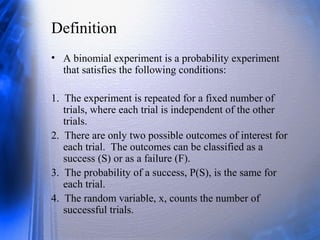
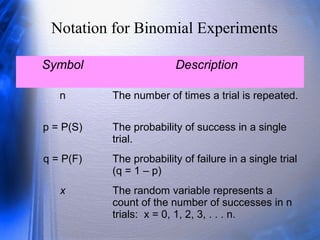
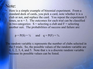
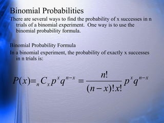
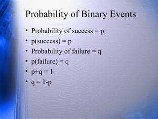
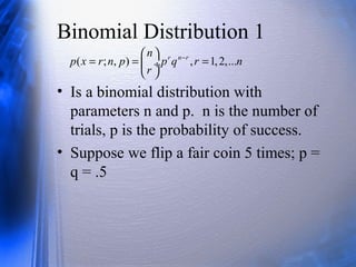
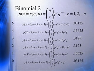
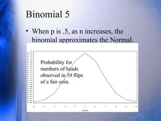
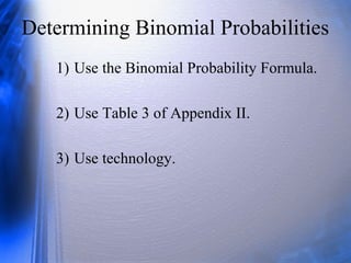
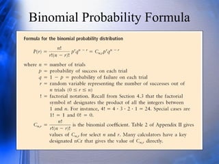
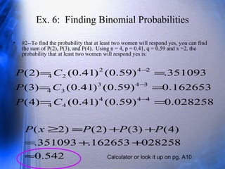
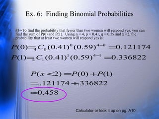
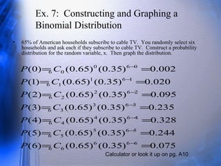
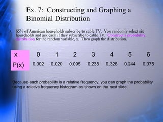
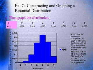
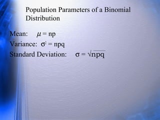
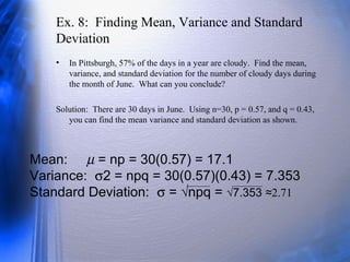
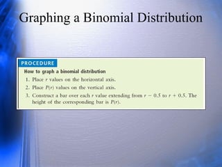
This document provides information about the binomial distribution including: - The conditions that define a binomial experiment with parameters n, p, and q - How to calculate binomial probabilities using the formula or tables - How to construct a binomial distribution and graph it - The mean, variance, and standard deviation of a binomial distribution are np, npq, and sqrt(npq) respectively

1. Binomial Distribution

2. Objectives/Assignment
• How to determine if a probability experiment
is a binomial experiment
• How to find binomial probabilities using the
binomial probability table and technology
• How to construct a binomial distribution and
its graph
• How to find the mean, variance and standard
deviation of a binomial probability
distribution
Assignment: pp. 173-175 #1-18 all

3. Binomial Experiments
• There are many probability experiments
for which the results of each trial can be
reduced to two outcomes: success and
failure. For instance, when a basketball
player attempts a free throw, he or she
either makes the basket or does not.
Probability experiments such as these
are called binomial experiments.

4. Definition
• A binomial experiment is a probability experiment
that satisfies the following conditions:
1. The experiment is repeated for a fixed number of
trials, where each trial is independent of the other
trials.
2. There are only two possible outcomes of interest for
each trial. The outcomes can be classified as a
success (S) or as a failure (F).
3. The probability of a success, P(S), is the same for
each trial.
4. The random variable, x, counts the number of
successful trials.

5. Notation for Binomial Experiments
Symbol Description
n The number of times a trial is repeated.
p = P(S) The probability of success in a single
trial.
q = P(F) The probability of failure in a single trial
(q = 1 – p)
x The random variable represents a
count of the number of successes in n
trials: x = 0, 1, 2, 3, . . . n.

6. Note:
• Here is a simple example of binomial experiment. From a
standard deck of cards, you pick a card, note whether it is a
club or not, and replace the card. You repeat the experiment 5
times, so n = 5. The outcomes for each trial can be classified
in two categories: S = selecting a club and F = selecting
another suit. The probabilities of success and failure are:
p = P(S) = ¼ and q = P(F) = ¾.
The random variable x represents the number of clubs selected in
the 5 trials. So, the possible values of the random variable are
0, 1, 2, 3, 4, and 5. Note that x is a discrete random variable
because its possible values can be listed.

7. Ex. 1: Binomial Experiments
• Decide whether the experiment is a binomial
experiment. If it is, specify the values of n, p
and q and list the possible values of the
random variable, x. If it is not, explain why.
1. A certain surgical procedure has an 85%
chance of success. A doctor performs the
procedure on eight patients. The random
variable represents the number of successful
surgeries.

8. Ex. 1: Binomial Experiments
Solution: the experiment is a binomial experiment
because it satisfies the four conditions of a binomial
experiment. In the experiment, each surgery
represents one trial. There are eight surgeries, and
each surgery is independent of the others. Also, there
are only two possible outcomes for each surgery—
either the surgery is a success or it is a failure.
Finally, the probability of success for each surgery is
0.85.
n = 8
p = 0.85
q = 1 – 0.85 = 0.15
x = 0, 1, 2, 3, 4, 5, 6, 7, 8

9. Ex. 1: Binomial Experiments
• Decide whether the experiment is a binomial
experiment. If it is, specify the values of n, p
and q and list the possible values of the
random variable, x. If it is not, explain why.
2. A jar contains five red marbles, nine blue
marbles and six green marbles. You randomly
select three marbles from the jar, without
replacement. The random variable represents
the number of red marbles.

10. Ex. 1: Binomial Experiments
Solution: The experiment is not a binomial
experiment because it does not satisfy all four
conditions of a binomial experiment. In the
experiment, each marble selection represents
one trial and selecting a red marble is a
success. When selecting the first marble, the
probability of success is 5/20. However
because the marble is not replaced, the
probability is no longer 5/20. So the trials are
not independent, and the probability of a
success is not the same for each trial.

11. Binomial Probabilities
There are several ways to find the probability of x successes in n
trials of a binomial experiment. One way is to use the
binomial probability formula.
Binomial Probability Formula
In a binomial experiment, the probability of exactly x successes
in n trials is:
xnxxnx
xn qp
xxn
n
qpCxP −−
−
==
!)!(
!
)(

12. Probability of Binary Events
• Probability of success = p
• p(success) = p
• Probability of failure = q
• p(failure) = q
• p+q = 1
• q = 1-p

13. Binomial Distribution 1
• Is a binomial distribution with
parameters n and p. n is the number of
trials, p is the probability of success.
• Suppose we flip a fair coin 5 times; p =
q = .5
( ; , ) , 1,2,...r n rn
p x r n p p q r n
r
− 
= = = ÷
 

14. Binomial 2
( ; , ) , 1,2,...r n rn
p x r n p p q r n
r
− 
= = = ÷
 
5 .03125
4 .15625
3 .3125
2 .3125
1 .15625
0 .03125
5 0 55
( 5; 5, .5) (1).5 (1)
5
p X n p p q
 
= = = = = ÷
 
4 1 45
( 4; 5, .5) 5
4
p X n p p q p q
 
= = = = = ÷
 
3 2 3 25
( 3; 5, .5) 10
3
p X n p p q p q
 
= = = = = ÷
 
2 3 2 35
( 2; 5, .5) 10
2
p X n p p q p q
 
= = = = = ÷
 
1 4 1 45
( 1; 5, .5) 5
1
p X n p p q p q
 
= = = = = ÷
 
0 5 55
( 0; 5, .5)
0
p X n p p q q
 
= = = = = ÷
 

15. Binomial 5
• When p is .5, as n increases, the
binomial approximates the Normal.
p
0. 00
0. 01
0. 02
0. 03
0. 04
0. 05
0. 06
0. 07
0. 08
0. 09
0. 10
0. 11
0. 12
0. 13
0. 14
0. 15
0. 16
0. 17
0. 18
0. 19
0. 20
0. 21
0. 22
0. 23
0. 24
0. 25
heads
0 1 2 3 4 5 6 7 8 9 10
Probability for
numbers of heads
observed in 10 flips
of a fair coin.

16. Determining Binomial Probabilities
1) Use the Binomial Probability Formula.
2) Use Table 3 of Appendix II.
3) Use technology.

17. Binomial Probability Formula

18. Using the Binomial Table
1) Locate the number of trials, n.
2) Locate the number of successes, r.
3) Follow that row to the right to the
corresponding p column.

19. Recall for the sharpshooter example, n = 8, r = 6, p = 0.7
So the probability she hits exactly 6 targets is 0.296, as expected

20. Binomial Probabilities
• At times, we will need to calculate other
probabilities:
– P(r < k)
– P(r ≤ k)
– P(r > k)
– P(r ≥ k)
Where k is a specified value less than or equal to
the number of trials, n.

21. Ex. 6: Finding Binomial Probabilities
• A survey indicates that 41% of
American women consider reading as
their favorite leisure time activity. You
randomly select four women and ask
them if reading is their favorite leisure-
time activity. Find the probability that
(1) exactly two of them respond yes, (2)
at least two of them respond yes, and
(3) fewer than two of them respond yes.

22. Ex. 6: Finding Binomial Probabilities
• #1--Using n = 4, p = 0.41, q = 0.59 and x =2, the probability
that exactly two women will respond yes is:
35109366.)3481)(.1681(.6
)3481)(.1681(.
4
24
)59.0()41.0(
!2)!24(
!4
)59.0()41.0()2(
242
242
24
=
=
=
−
==
−
−
CP
Calculator or look it up on pg. A10

23. Ex. 6: Finding Binomial Probabilities
• #2--To find the probability that at least two women will respond yes, you can find
the sum of P(2), P(3), and P(4). Using n = 4, p = 0.41, q = 0.59 and x =2, the
probability that at least two women will respond yes is:
028258.0)59.0()41.0()4(
162653.0)59.0()41.0()3(
351093.)59.0()41.0()2(
444
44
343
34
242
24
==
==
==
−
−
−
CP
CP
CP
542.0
028258162653.351093.
)4()3()2()2(
≈
++=
++=≥ PPPxP
Calculator or look it up on pg. A10

24. Ex. 6: Finding Binomial Probabilities
• #3--To find the probability that fewer than two women will respond yes, you can
find the sum of P(0) and P(1). Using n = 4, p = 0.41, q = 0.59 and x =2, the
probability that at least two women will respond yes is:
336822.0)59.0()41.0()1(
121174.0)59.0()41.0()0(
141
14
040
04
==
==
−
−
CP
CP
458.0
336822.121174..
)1()0()2(
≈
+=
+=< PPxP
Calculator or look it up on pg. A10

25. Ex. 7: Constructing and Graphing a
Binomial Distribution
• 65% of American households subscribe to cable TV. You randomly select six
households and ask each if they subscribe to cable TV. Construct a probability
distribution for the random variable, x. Then graph the distribution.
Calculator or look it up on pg. A10
075.0)35.0()65.0()6(
244.0)35.0()65.0()5(
328.0)35.0()65.0()4(
235.0)35.0()65.0()3(
095.0)35.0()65.0()2(
020.0)35.0()65.0()1(
002.0)35.0()65.0()0(
666
66
565
56
464
46
363
36
262
26
161
16
060
06
==
==
==
==
==
==
==
−
−
−
−
−
−
−
CP
CP
CP
CP
CP
CP
CP

26. Ex. 7: Constructing and Graphing a
Binomial Distribution
• 65% of American households subscribe to cable TV. You randomly select six
households and ask each if they subscribe to cable TV. Construct a probability
distribution for the random variable, x. Then graph the distribution.
Because each probability is a relative frequency, you can graph the probability
using a relative frequency histogram as shown on the next slide.
x 0 1 2 3 4 5 6
P(x) 0.002 0.020 0.095 0.235 0.328 0.244 0.075

27. Ex. 7: Constructing and Graphing a
Binomial Distribution
• Then graph the distribution.
x 0 1 2 3 4 5 6
P(x) 0.002 0.020 0.095 0.235 0.328 0.244 0.075
0
0.05
0.1
0.15
0.2
0.25
0.3
0.35
0 1 2 3 4 5 6
P(x)
R
e
l
a
t
i
v
e
F
r
e
q
u
e
n
c
y
Households
NOTE: that the
histogram is
skewed left. The
graph of a binomial
distribution with p >
.05 is skewed left,
while the graph of a
binomial
distribution with p <
.05 is skewed right.
The graph of a
binomial
distribution with p =
.05 is symmetric.

28. Population Parameters of a Binomial
Distribution
Mean: µ = np
Variance: σ2
= npq
Standard Deviation: σ = √npq

29. Ex. 8: Finding Mean, Variance and Standard
Deviation
• In Pittsburgh, 57% of the days in a year are cloudy. Find the mean,
variance, and standard deviation for the number of cloudy days during
the month of June. What can you conclude?
Solution: There are 30 days in June. Using n=30, p = 0.57, and q = 0.43,
you can find the mean variance and standard deviation as shown.
Mean: µ = np = 30(0.57) = 17.1
Variance: σ2 = npq = 30(0.57)(0.43) = 7.353
Standard Deviation: σ = √npq = √7.353 2.71≈

30. Graphing a Binomial Distribution

31. Critical Thinking
• Unusual values – For a binomial
distribution, it is unusual for the
number of successes r to be more than
2.5 standard deviations from the mean.
– This can be used as an indicator to
determine whether a specified number
of r out of n trials in a binomial
experiment is unusual.

32. 1 2 1 1 2 1
2 1
!
( )
( )! !
2!
(1) 0.4 0.6 0.4 0.6 2*0.4*0.6 0.48
(2 1)!1!
x n x x n x
n x
n
P x C p q p q
n x x
P C
− −
− −
= =
−
= = = =
−