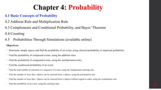
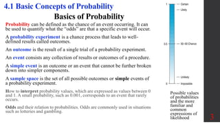
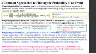
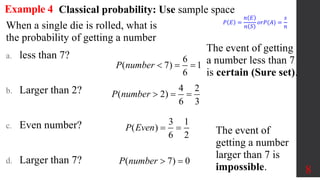
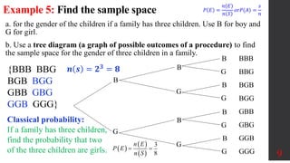
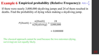
Please Subscribe to this Channel for more solutions and lectures http://www.youtube.com/onlineteaching Chapter 4: Probability 4.1: Basic Concepts of Probability

1. Elementary Statistics
Chapter 4:
Probability
4.1 Basic Concepts of
probability
1

2. Chapter 4: Probability
4.1 Basic Concepts of Probability
4.2 Addition Rule and Multiplication Rule
4.3 Complements and Conditional Probability, and Bayes’ Theorem
4.4 Counting
4.5 Probabilities Through Simulations (available online)
2
Objectives:
• Determine sample spaces and find the probability of an event, using classical probability or empirical probability.
• Find the probability of compound events, using the addition rules.
• Find the probability of compound events, using the multiplication rules.
• Find the conditional probability of an event.
• Find the total number of outcomes in a sequence of events, using the fundamental counting rule.
• Find the number of ways that r objects can be selected from n objects, using the permutation rule.
• Find the number of ways that r objects can be selected from n objects without regard to order, using the combination rule.
• Find the probability of an event, using the counting rules.

3. Basics of Probability
Probability can be defined as the chance of an event occurring. It can
be used to quantify what the “odds” are that a specific event will occur.
A probability experiment is a chance process that leads to well-
defined results called outcomes.
An outcome is the result of a single trial of a probability experiment.
An event consists any collection of results or outcomes of a procedure.
A simple event is an outcome or an event that cannot be further broken
down into simpler components.
A sample space is the set of all possible outcomes or simple events of
a probability experiment.
How to interpret probability values, which are expressed as values between 0
and 1. A small probability, such as 0.001, corresponds to an event that rarely
occurs.
Odds and their relation to probabilities. Odds are commonly used in situations
such as lotteries and gambling.
3
4.1 Basic Concepts of Probability
Possible values
of probabilities
and the more
familiar and
common
expressions of
likelihood

4. Example 1
4
4.1 Basic Concepts of Probability
Sample Spaces
Experiment Sample Space
Toss a coin Head, Tail
Roll a die 1, 2, 3, 4, 5, 6
Answer a true/false
question
True, False
Toss two coins HH, HT, TH, TT

5. Example 2 Simple Events and Sample Spaces
Use “b” to denote a baby boy and “g” to denote a baby girl.
5
Procedure /
Experiment
Example of Event
Sample Space: Complete List of
Simple Events
Single birth 1 girl (simple event) {b, g}
3 births 2 boys and 1 girl (bbg, bgb, and gbb are all simple
events resulting in 2 boys and 1 girl)
{bbb, bbg, bgb, bgg, gbb, gbg, ggb,
ggg}
Simple Events:
1 birth: The result of 1 girl is a simple event and so is the result of 1 boy.
3 births: The result of 2 girls followed by a boy (ggb) is a simple event.
3 births: The event of “2 girls and 1 boy” is not a simple event because it can
occur with these different simple events: ggb, gbg, bgg. It is a compound event.
3 births: The sample space consists of the eight (23
) different simple events
listed in the above table.

6. Example 3: Find the sample space
6
a. for rolling one die.
b. for rolling two dice.
n(s) = 6 Outcomes:
1, 2, 3, 4, 5, 6
𝒏 𝒔 = 𝟔𝟐
= 𝟑𝟔
𝒏 𝒔 = (# 𝒐𝒇 𝒐𝒖𝒕𝒄𝒐𝒎𝒆𝒔)# 𝒐𝒇 𝒔𝒕𝒂𝒈𝒆𝒔
Probability Warm up: What is the probability
of getting “snake-eyes” (two 1’s)?

7. 3 Common Approaches to Finding the Probability of an Event
•Classical probability uses sample spaces to determine the numerical probability that an event will
happen and assumes that all outcomes in the sample space are equally likely to occur. (confirm that the
outcomes are equally likely)
•Empirical probability (Relative Frequency Approximation of Probability) Conduct (or observe) a
procedure and count the number of times that event A occurs. P(A) is then approximated as follows:
•Subjective probability: P(A), the probability of event A, is estimated by using knowledge of the
relevant circumstances. (A subjective probability can be estimated in the absence of historical data.) uses
a probability value based on an educated guess or estimate, employing opinions and inexact information.
Experiments that have neither equally likely outcomes nor the potential of being repeated are assigned by
subjective probability. Examples: weather forecasting, predicting outcomes of sporting events
•Simulations: Sometimes none of the preceding three approaches can be used. A simulation of a
procedure is a process that behaves in the same ways as the procedure itself so that similar results are
produced. Probabilities can sometimes be found by using a simulation. 7
𝑃 𝐸 =
𝑛 𝐸
𝑛 𝑆
=
# of desired outcomes
Total # of possible outcomes
, 𝑜𝑟𝑃(𝐴) =
𝑠
𝑛
𝑃(𝐴) =
𝑛(𝐴)
𝑛(Procedure Repeated)
, 𝑂𝑟𝑃 𝐸 =
𝑓
𝑛
=
frequency of desired class
Sum of all frequencies
Example:
P (Even numbers in roll of a die) =
3
6
=
1
2
Example: P (A randomly selected student
from a Statistics class is a female) =
𝑁𝑢𝑚𝑏𝑒𝑟 𝑜𝑓 𝑓𝑒𝑚𝑎𝑙𝑒 𝑠𝑡𝑢𝑑𝑒𝑛𝑡𝑠
𝑇𝑜𝑡𝑎𝑙

8. 8
Example 4
When a single die is rolled, what is
the probability of getting a number
a. less than 7?
b. Larger than 2?
c. Even number?
d. Larger than 7?
6
( 7) 1
6
P number   
The event of getting
a number less than 7
is certain (Sure set).
4 2
( 2)
6 3
P number   
3 1
( )
6 2
P Even  
( 7) 0
P number  
Classical probability: Use sample space
𝑃 𝐸 =
𝑛 𝐸
𝑛 𝑆
𝑜𝑟𝑃(𝐴) =
𝑠
𝑛
The event of
getting a number
larger than 7 is
impossible.

9. Example 5: Find the sample space
9
a. for the gender of the children if a family has three children. Use B for boy and
G for girl.
b. Use a tree diagram (a graph of possible outcomes of a procedure) to find
the sample space for the gender of three children in a family.
{BBB BBG
BGB BGG
GBB GBG
GGB GGG}
𝒏 𝒔 = 𝟐𝟑
= 𝟖
B
G
B
G
B
G
B
G
B
G
B
G
B
G
BBB
BBG
BGB
BGG
GBB
GBG
GGB
GGG
Classical probability:
If a family has three children,
find the probability that two
of the three children are girls.  
 
 
3
8
n E
P E
n S
 
𝑃 𝐸 =
𝑛 𝐸
𝑛 𝑆
𝑜𝑟𝑃(𝐴) =
𝑠
𝑛

10. Example 6
If there were nearly 3,000,000 skydiving jumps and 24 of them resulted in
deaths. Find the probability of dying when making a skydiving jump.
10
The classical approach cannot be used because the two outcomes (dying,
surviving) are not equally likely.
𝑃(𝐷𝑒𝑎𝑡ℎ) =
𝑛(𝐷𝑒𝑎𝑡ℎ)
𝑛(𝑆𝑘𝑦𝑑𝑖𝑣𝑖𝑛𝑔)
=
24
3,000,000
= 0.000008
Empirical probability (Relative Frequency): 𝑃 𝐸 =
𝑓
𝑛

11. Example 7
In a high school, it was found that 450 of them texted while driving in a
semester, and 550 did not do so. According to these results, if a high
school driver is randomly selected, find the probability that he or she
texted while driving during the same time period.
11
𝑃(𝑇𝑒𝑥𝑡𝑖𝑛𝑔) =
𝑛(𝑇𝑒𝑥𝑡𝑒𝑟𝑠)
𝑛(𝐷𝑟𝑖𝑣𝑒𝑟𝑠)
=
450
1000
= 0.45
Interpretation: There is a 0.45 probability that if a high school driver is randomly
selected, he or she texted while driving during the last semester.
Texted
Did not
text
450 550
Empirical probability (Relative Frequency): 𝑃 𝐸 =
𝑓
𝑛

12. Example 8
In a sample of 50 people, 21 had type O blood, 22 had type A blood, 5 had
type B blood, and 2 had type AB blood. Set up a frequency distribution and
find the following probabilities.
a. A person has type O blood.
b. A person has type A or type B blood.
c. A person has neither type A nor type O blood.
d. A person does not have type AB blood.
12
Empirical probability (Relative Frequency): 𝑃 𝐸 =
𝑓
𝑛
Type Frequency
A 22
B 5
AB 2
O 21
Total 50
𝑎. 𝑃 O =
𝑓
𝑛
=
21
50
𝑏. 𝑃 A or B =
22
50
+
5
50
=
27
50
𝑐.
𝑃 neither A nor O
=
5
50
+
2
50
=
7
50
𝑑. 𝑃 not AB = 1 − 𝑃 AB = 1 −
2
50
=
48
50
=
24
25

13. Complementary Events:
13
P A = 1 − P A
Example 9
Find the complement of each event.
Event Complement of the Event
Rolling a die and getting a 4 Getting a 1, 2, 3, 5, or 6
Selecting a letter of the alphabet
and getting a vowel
Getting a consonant (assume y is a
consonant)
Selecting a month and getting a
month that begins with a J
Getting February, March, April,
May, August, September, October,
November, or December
Selecting a day of the week
and getting a weekday Getting Saturday or Sunday

14. Complementary Events:
The complement of an eventA, denoted by 𝐴, consists of all outcomes that are not included in the
outcomes of eventA.
14
P A = 1 − P A
Example 10
If there were nearly 3,000,000 skydiving jumps and 24 of them resulted in death.
Find the probability of not dying when making a skydiving jump.
Example 11: In reality, more boys are born than girls. In one typical group,
there are 205 newborn babies, 105 of whom are boys. If one baby is randomly
selected from the group, what is the probability that the baby is not a boy?
Recall: 𝑃(𝐷𝑒𝑎𝑡ℎ) = 0.000008
= 1 − 0.000008 = 0.999992
𝑃(𝑁𝑜𝑡 − 𝐷𝑦𝑖𝑛𝑔) = 1 − 𝑃(𝐷𝑒𝑎𝑡ℎ)
P B = 1 − P B = 𝑃(𝐺) =
100
205
= 0.488

15. 15
4.1 Basic Concepts of Probability, Odds
The actual odds against event A occurring are the ratio O 𝐴 =
𝑃 𝐴
𝑃(𝐴)
, usually
expressed in the form of a:b (or “a to b”), where a and b are integers having no
common factors.
The actual odds in favor event A occurring are the reciprocal of the actual odds
against the event. If the odds against A are a:b, then the odds in favor of A are b:a.
The payoff odds against event A represent the ratio of the net profit (if you win) to the
amount bet.
Payoff odds against event A = (net profit):(amount bet)
Payoff odds against event A =
net profit
amount bet
net profit = (Payoff odds against event A)(amount bet)

16. Example 12
16
If you bet $5 on the number 13 in roulette, your probability of winning is 1/38, but
your payoff odds are given be casino as 35:1.
a. Find the actual odds against the outcome of 13.
b. How much net profit would you make if you win by betting $5 on 13?
c. If the casino was not operating for profit and the payoff odds were changed to match
the actual odds against 13, how much would you win if the outcome were 13?
O 𝐴 =
𝑃 𝐴
𝑃(𝐴)
O 𝐴 =
𝑃 𝐴
𝑃(𝐴)
=
1 − 1/38
1/38
=
37/38
1/38
=
37
1
b. 35:1 = (net profit):(amount bet)
net profit = Payoff odds against event A amount bet
= 35 $5 = $175
The winner collects: $175 + the original $5 bet = $180, for a net profit of $175.
c. If the casino were not operating for profit, the payoff odds = 37:1 (Net profit of
$37 for each $1 bet) : net profit = 37 $5 = $185
(The casino makes its profit by providing a profit of only $175 instead of the $185
that would be paid with a roulette game that is fair instead of favoring the casino.)
Payoff odds against event A =
net profit
amount bet

17. Law of Large Numbers & Identifying Significant Results with Probabilities
The Rare Event Rule for Inferential Statistics
If, under a given assumption, the probability of a particular observed event is very small and the observed event occurs significantly less than or
significantly greater than what we typically expect with that assumption, we conclude that the assumption is probably not correct.
Using Probabilities to Determine When Results Are Significantly High or Significantly Low
Significantly high number of successes: x successes among n trials is a significantly high number of successes if the probability of x or more
successes is unlikely with a probability of 0.05 or less. That is, x is a significantly high number of successes if P(x or more) ≤ 0.05*.
Significantly low number of successes: x successes among n trials is a significantly low number of successes if the probability of x or fewer
successes is unlikely with a probability of 0.05 or less. That is, x is a significantly low number of successes if P(x or fewer) ≤ 0.05*.
*The value 0.05 is not absolutely rigid.
17
Law of Large Numbers:
As a procedure is repeated again and again, the relative frequency probability of an
event tends to approach the actual probability, and it applies to behavior over a large
number of trials, and it does not apply to any one individual outcome.
Example: Observation: A coin is tossed 100 times and we get 98 heads in a row.
Assumption: The coin is fair. (a normal assumption when an ordinary coin is tossed)
If the assumption is true, we have observed a highly unlikely event.
According to The Rare Event Rule , therefore, what we just observed is evidence against the assumption.
On this basis, we conclude the assumption is wrong (the coin is loaded.)