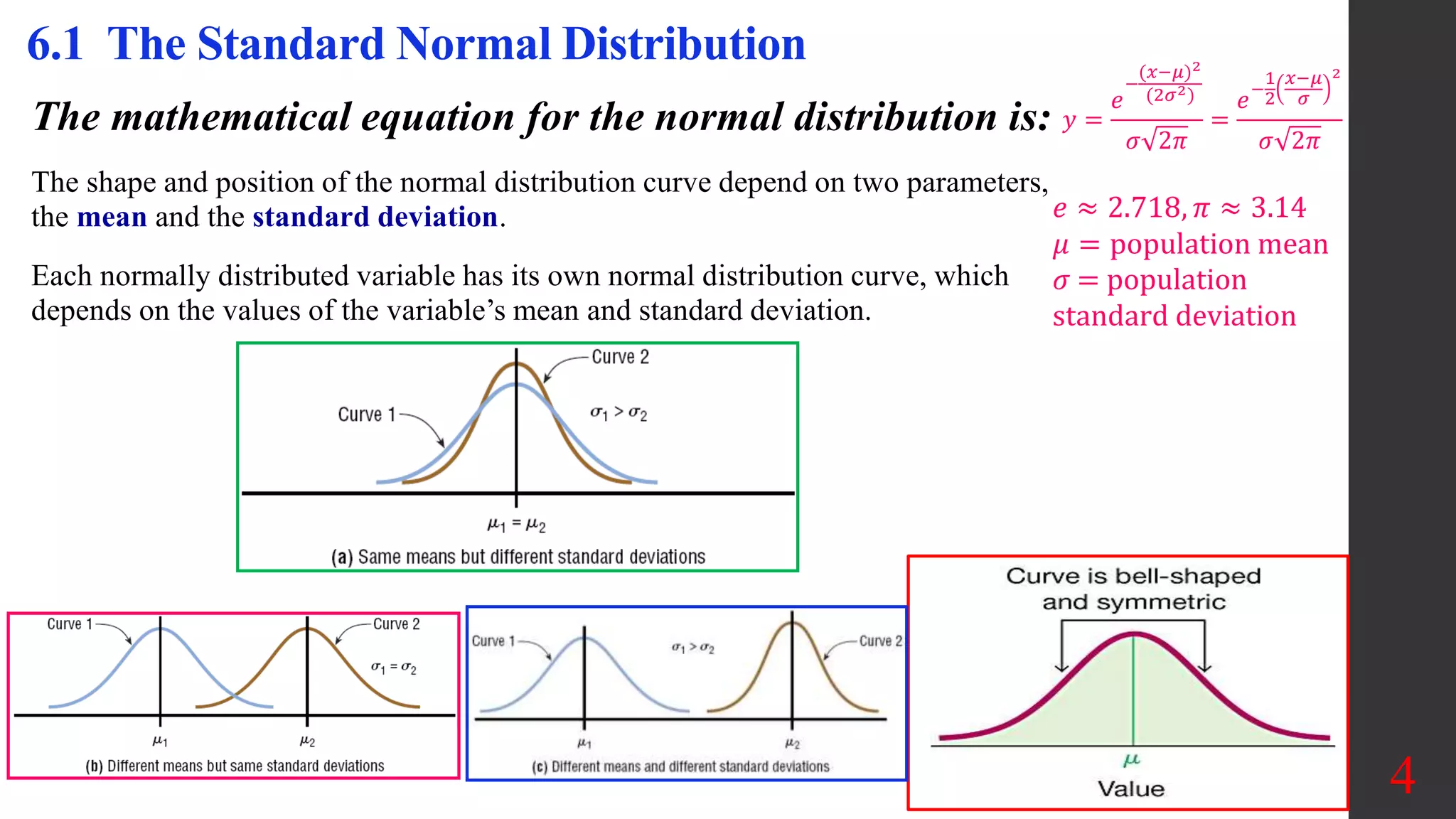
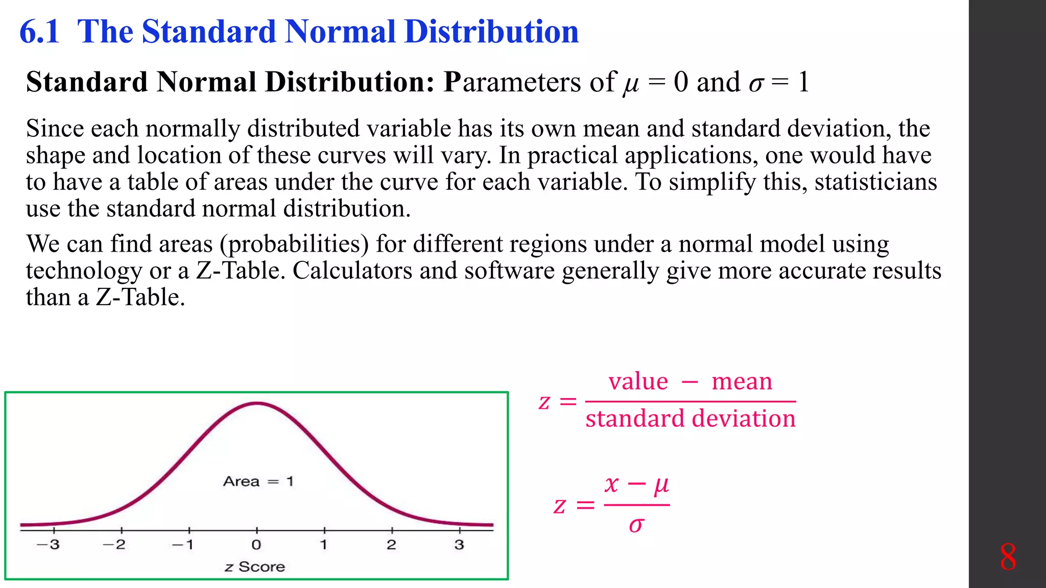
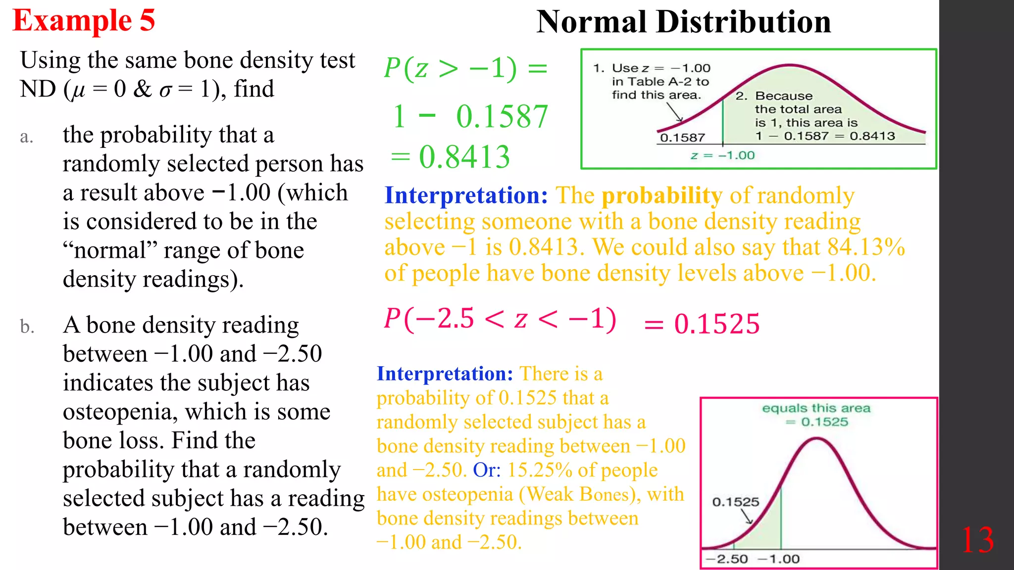
SlideShare a Scribd company logo
1 of 16
Elementary Statistics
Chapter 6:
Normal Probability
Distribution
6.1 The Standard
Normal Distribution
1
Chapter 6: Normal Probability Distribution
6.1 The Standard Normal Distribution
6.2 Real Applications of Normal Distributions
6.3 Sampling Distributions and Estimators
6.4 The Central Limit Theorem
6.5 Assessing Normality
6.6 Normal as Approximation to Binomial
2
Objectives:
• Identify distributions as symmetric or skewed.
• Identify the properties of a normal distribution.
• Find the area under the standard normal distribution, given various z values.
• Find probabilities for a normally distributed variable by transforming it into a standard normal variable.
• Find specific data values for given percentages, using the standard normal distribution.
• Use the central limit theorem to solve problems involving sample means for large samples.
• Use the normal approximation to compute probabilities for a binomial variable.
6.1 The Standard Normal Distribution
Normal Distribution
If a continuous random variable has a distribution with a graph that is
symmetric and bell-shaped, we say that it has a normal distribution.
3
Key Concept: the standard normal distribution is a specific normal distribution having
the following three properties:
1. Bell-shaped: The graph of the standard normal distribution is bell-shaped.
2. µ = 0: The standard normal distribution has a mean equal to 0.
3. σ = 1: The standard normal distribution has a standard deviation equal to 1.
In this section we develop the skill to find areas (or probabilities or relative frequencies)
corresponding to various regions under the graph of the standard normal distribution. In
addition, we find z scores that correspond to areas under the graph.
For a continuous random variable, the probability of a single value of x is always zero.
The mathematical equation for the normal distribution is:
The shape and position of the normal distribution curve depend on two parameters,
the mean and the standard deviation.
Each normally distributed variable has its own normal distribution curve, which
depends on the values of the variable’s mean and standard deviation.
4
6.1 The Standard Normal Distribution
𝑒 ≈ 2.718, 𝜋 ≈ 3.14
𝜇 = population mean
𝜎 = population
standard deviation
𝑦 =
𝑒
−
(𝑥−𝜇)2
(2𝜎2)
𝜎 2𝜋
=
𝑒
−
1
2
𝑥−𝜇
𝜎
2
𝜎 2𝜋
• The normal distribution curve is bell-shaped.
• The mean, median, and mode are equal and located at the center of the distribution.
• The normal distribution curve is Unimodal (i.e., it has only one mode).
• The curve is symmetrical about the mean, which is equivalent to saying that its shape
is the same on both sides of a vertical line passing through the center.
• The curve is continuous—i.e., there are no gaps or holes.
• The curve never touches the x-axis. Theoretically, no matter how far in either
direction the curve extends, it never meets the x-axis—but it gets increasingly
closer.
• The total area under the curve = 1.00 or 100%.
• The area under the normal curve that lies within
 one standard deviation of the mean is approximately 0.68 (68%).
 two standard deviations of the mean is approximately 0.95 (95%).
 three standard deviations of the mean is approximately 0.997 ( 99.7%).
5
6.1 The Standard Normal Distribution
𝑦 =
𝑒
−
(𝑥−𝜇)2
(2𝜎2)
𝜎 2𝜋
Uniform Distribution
A continuous random variable has a uniform distribution if its values are spread evenly
over the range of possibilities. The graph of a uniform distribution results in a rectangular
shape.
Properties of uniform distribution:
1. The area under the graph of a continuous probability distribution is equal to 1.
2. There is a correspondence between area and probability, so probabilities can be found by
identifying the corresponding areas in the graph using this formula for the area of a
rectangle:
Area = height × width
Density Curve:
 The graph of any continuous probability distribution is called a density curve, and any
density curve must satisfy the requirement that the total area under the curve is exactly 1.
Because the total area under any density curve is equal to 1, there is a correspondence
between area and probability.
6
Uniform Distribution
6.1 The Standard Normal Distribution
Example 1
At JFK airport in New York City, passengers arriving at the security checkpoint
have waiting times that are uniformly distributed between 0 minutes and 5
minutes. All of the different possible waiting times are equally likely. Waiting
times can be any value between 0 min and 5 min (it’s a continuous value), so it
is possible to have a waiting time of 1.234567 min. Find the probability that a
randomly selected passenger has a waiting time of at least 2 minutes.
7
Uniform Distribution
Given: The total area under the curve = 1.00, 𝑤𝑖𝑑𝑡ℎ = 5
Height (the probability) =
1
𝑤𝑖𝑑𝑡ℎ
→ ℎ =
1
5
= 0.2
Solution: P(wait time of at least 2 min) = P x ≥ 2 =
= height × width of shaded area in the figure = 0.2 × 3 = 0.6
Standard Normal Distribution: Parameters of µ = 0 and σ = 1
Since each normally distributed variable has its own mean and standard deviation, the
shape and location of these curves will vary. In practical applications, one would have
to have a table of areas under the curve for each variable. To simplify this, statisticians
use the standard normal distribution.
We can find areas (probabilities) for different regions under a normal model using
technology or a Z-Table. Calculators and software generally give more accurate results
than a Z-Table.
8
6.1 The Standard Normal Distribution
𝑧 =
value − mean
standard deviation
𝑧 =
𝑥 − 𝜇
𝜎
Formats Used for Finding Normal Distribution Areas
9
1. To the left of any z
value: Look up the z value in the
table and use the area given.
2. To the right of any
z value: Look up the z value
and subtract the area from 1.
3. Between two
z values: Look up
both z values and
subtract the
corresponding areas.
A bone mineral density test can help identify the presence or likelihood of osteoporosis
which is measured as a z score: ND (µ = 0 & σ = 1).
Q: A randomly selected adult undergoes a bone density test. Find the probability that
this person has a bone density test score less than 1.27.
10
Example 2 Normal Distribution
Locate 1.2 in the left column and 0.07 in the top row: Read the value
Interpretation: The probability that a randomly selected person
has a bone density test result below 1.27 is 0.8980 (Or: Conclude
that 89.80% of people have bone density levels below 1.27.
𝑃(𝑧 < 1.27) = 0.8980
P(a < z < b) denotes the probability that the z score is between a and b.
P(z > a) denotes the probability that the z score is greater than a.
P(z < a) denotes the probability that the z score is less than a.
11
SND: Standard Normal Distribution
Finding Areas from the z Scores
a. Find the area to the left of z = 2.06.
b. Find the area to the right of z = –1.19.
Example 3
𝑃(𝑧 < 2.06) = 0.9803
𝑃(𝑧 > −1.19) = 0.8830
TI Calculator:
Normal Distribution Area
1. 2nd + VARS
2. normalcdf(
3. 4 entries required
4. Left bound, Right
bound, value of the
Mean, Standard
deviation
5. Enter
6. For −∞, 𝒖𝒔𝒆 − 𝟏𝟎𝟎𝟎
7. For ∞, 𝒖𝒔𝒆 𝟏𝟎𝟎𝟎
12
a. Find the area between z = +1.68 and z = –1.37.
b. Find the probability: P(0 < z < 2.32)
Example 4 SND: Standard Normal Distribution
𝑃(0 < 𝑧 < 2.32) =
𝑃(−1.37 < 𝑧 < 1.68) =
0.9535 − 0.0853 = 0.8682
= 0.9898 − 0.5 = 0.4898
Using the same bone density test
ND (µ = 0 & σ = 1), find
a. the probability that a
randomly selected person has
a result above −1.00 (which
is considered to be in the
“normal” range of bone
density readings).
b. A bone density reading
between −1.00 and −2.50
indicates the subject has
osteopenia, which is some
bone loss. Find the
probability that a randomly
selected subject has a reading
between −1.00 and −2.50.
13
Example 5 Normal Distribution
1 − 0.1587
= 0.8413
𝑃(𝑧 > −1) =
Interpretation: The probability of randomly
selecting someone with a bone density reading
above −1 is 0.8413. We could also say that 84.13%
of people have bone density levels above −1.00.
𝑃(−2.5 < 𝑧 < −1) = 0.1525
Interpretation: There is a
probability of 0.1525 that a
randomly selected subject has a
bone density reading between −1.00
and −2.50. Or: 15.25% of people
have osteopenia (Weak Bones), with
bone density readings between
−1.00 and −2.50.
Notation & Finding z Scores from Known Areas
14
Draw a bell-shaped curve and identify the region under the curve that
corresponds to the given probability. If that region is not a cumulative region
from the left, work instead with a known region that is a cumulative region
from the left.
Use technology or the Z-Table find the z score. With Table A-2, use the
cumulative area from the left, locate the closest probability in the body of the
table, and identify the corresponding z score.
Critical Value: For the standard normal distribution, a critical value is a z
score on the borderline separating those z scores that are significantly low or
significantly high.
Notation: The expression zα denotes the z score with an area of α to its right.
Find the value of z0.025. (Let α = 0.025 in the expression zα.)
15
Example 6 Normal Distribution
Solution
The notation of z0.025 is used to represent the z score with an area of 0.025 to its right.
Note: that the value of z = 1.96 has an area of 0.025 to its right, so z0.025 = 1.96.
Note that z0.025 corresponds to a cumulative left area of 0.975.
CAUTION:
When finding a value of zα for a particular value of α, note that α is the area to the right of zα,
but the Table and some technologies give cumulative areas to the left of a given z score. To
find the value of zα, resolve that conflict by using the value of 1 − α. For example, to find z0.1,
refer to the z score with an area of 0.9 to its left.
TI Calculator:
Normal Distribution: find
the Z-score
1. 2nd + VARS
2. invNorm(
3. 3 entries required
4. Left Area, value of the
Mean, Standard
deviation
5. Enter
16
Find the z value such that
a. the area under the standard normal distribution
curve between 0 and the z value is 0.2123.
b. Find 𝑃10, the 10th percentile.
Example 7 SND: Standard Normal Distribution
𝑃(0 < 𝑧 < 𝑧 − 𝑣𝑎𝑙𝑢𝑒) = 0.2123
Add 0.5000 to 0.2123 to get the
cumulative area = 0.7123, why?
The z value is 0.56.
𝑃10 = −1.28, why?
Area = 𝟏𝟎% = 𝟎. 𝟏

More Related Content

What's hot

What's hot (20)

Assessing Normality
Assessing NormalityAssessing Normality
Assessing Normality
 
Probability Distribution
Probability DistributionProbability Distribution
Probability Distribution
 
Real Applications of Normal Distributions
Real Applications of Normal Distributions Real Applications of Normal Distributions
Real Applications of Normal Distributions
 
The normal distribution
The normal distributionThe normal distribution
The normal distribution
 
Normal distribution
Normal distributionNormal distribution
Normal distribution
 
Standard normal distribution
Standard normal distributionStandard normal distribution
Standard normal distribution
 
Review & Hypothesis Testing
Review & Hypothesis TestingReview & Hypothesis Testing
Review & Hypothesis Testing
 
Binomial Probability Distributions
Binomial Probability DistributionsBinomial Probability Distributions
Binomial Probability Distributions
 
Estimating a Population Standard Deviation or Variance
Estimating a Population Standard Deviation or Variance Estimating a Population Standard Deviation or Variance
Estimating a Population Standard Deviation or Variance
 
Testing a Claim About a Proportion
Testing a Claim About a ProportionTesting a Claim About a Proportion
Testing a Claim About a Proportion
 
Practice Test 1
Practice Test 1Practice Test 1
Practice Test 1
 
Poisson Probability Distributions
Poisson Probability DistributionsPoisson Probability Distributions
Poisson Probability Distributions
 
Two Means, Independent Samples
Two Means, Independent SamplesTwo Means, Independent Samples
Two Means, Independent Samples
 
Discrete distributions: Binomial, Poisson & Hypergeometric distributions
Discrete distributions:  Binomial, Poisson & Hypergeometric distributionsDiscrete distributions:  Binomial, Poisson & Hypergeometric distributions
Discrete distributions: Binomial, Poisson & Hypergeometric distributions
 
Probability Distributions for Discrete Variables
Probability Distributions for Discrete VariablesProbability Distributions for Discrete Variables
Probability Distributions for Discrete Variables
 
Geometric probability distribution
Geometric probability distributionGeometric probability distribution
Geometric probability distribution
 
Two Variances or Standard Deviations
Two Variances or Standard DeviationsTwo Variances or Standard Deviations
Two Variances or Standard Deviations
 
Probability Distribution
Probability DistributionProbability Distribution
Probability Distribution
 
Practice test ch 8 hypothesis testing ch 9 two populations
Practice test ch 8 hypothesis testing ch 9 two populationsPractice test ch 8 hypothesis testing ch 9 two populations
Practice test ch 8 hypothesis testing ch 9 two populations
 
Confidence Intervals
Confidence IntervalsConfidence Intervals
Confidence Intervals
 

Similar to The Standard Normal Distribution

Normal Probability Distribution
Normal Probability DistributionNormal Probability Distribution
Normal Probability Distribution
mandalina landy
 
Density Curves and Normal Distributions
Density Curves and Normal DistributionsDensity Curves and Normal Distributions
Density Curves and Normal Distributions
nszakir
 
Statistik 1 6 distribusi probabilitas normal
Statistik 1 6 distribusi probabilitas normalStatistik 1 6 distribusi probabilitas normal
Statistik 1 6 distribusi probabilitas normal
Selvin Hadi
 

Similar to The Standard Normal Distribution (20)

The Standard Normal Distribution
The Standard Normal Distribution  The Standard Normal Distribution
The Standard Normal Distribution
 
Real Applications of Normal Distributions
Real Applications of Normal Distributions  Real Applications of Normal Distributions
Real Applications of Normal Distributions
 
Normal Probability Distribution
Normal Probability DistributionNormal Probability Distribution
Normal Probability Distribution
 
St201 d normal distributions
St201 d normal distributionsSt201 d normal distributions
St201 d normal distributions
 
04.NORMAL DISTRIBUTION stat and probab.pptx
04.NORMAL DISTRIBUTION stat and probab.pptx04.NORMAL DISTRIBUTION stat and probab.pptx
04.NORMAL DISTRIBUTION stat and probab.pptx
 
Ch05
Ch05Ch05
Ch05
 
Lecture 01 probability distributions
Lecture 01 probability distributionsLecture 01 probability distributions
Lecture 01 probability distributions
 
Density Curves and Normal Distributions
Density Curves and Normal DistributionsDensity Curves and Normal Distributions
Density Curves and Normal Distributions
 
Statistik 1 6 distribusi probabilitas normal
Statistik 1 6 distribusi probabilitas normalStatistik 1 6 distribusi probabilitas normal
Statistik 1 6 distribusi probabilitas normal
 
Les5e ppt 05
Les5e ppt 05Les5e ppt 05
Les5e ppt 05
 
Les5e ppt 05
Les5e ppt 05Les5e ppt 05
Les5e ppt 05
 
Statistics and Probability- NORMAL DISTRIBUTION.pptx
Statistics and Probability- NORMAL DISTRIBUTION.pptxStatistics and Probability- NORMAL DISTRIBUTION.pptx
Statistics and Probability- NORMAL DISTRIBUTION.pptx
 
The-Normal-Distribution, Statics and Pro
The-Normal-Distribution, Statics and ProThe-Normal-Distribution, Statics and Pro
The-Normal-Distribution, Statics and Pro
 
4 2 continuous probability distributionn
4 2 continuous probability    distributionn4 2 continuous probability    distributionn
4 2 continuous probability distributionn
 
Normal as Approximation to Binomial
Normal as Approximation to Binomial  Normal as Approximation to Binomial
Normal as Approximation to Binomial
 
Ch3 Probability and The Normal Distribution
Ch3 Probability and The Normal Distribution Ch3 Probability and The Normal Distribution
Ch3 Probability and The Normal Distribution
 
8. normal distribution qt pgdm 1st semester
8. normal distribution qt pgdm 1st  semester8. normal distribution qt pgdm 1st  semester
8. normal distribution qt pgdm 1st semester
 
Chapter9 the normal curve distribution
Chapter9 the normal curve distributionChapter9 the normal curve distribution
Chapter9 the normal curve distribution
 
02 PSBE3_PPT.Ch01_2_Examining Distribution.ppt
02 PSBE3_PPT.Ch01_2_Examining Distribution.ppt02 PSBE3_PPT.Ch01_2_Examining Distribution.ppt
02 PSBE3_PPT.Ch01_2_Examining Distribution.ppt
 
Stats chapter 2
Stats chapter 2 Stats chapter 2
Stats chapter 2
 

More from Long Beach City College

More from Long Beach City College (20)

Practice test ch 9 inferences from two samples
Practice test ch 9 inferences from two samplesPractice test ch 9 inferences from two samples
Practice test ch 9 inferences from two samples
 
Practice Test Ch 8 Hypothesis Testing
Practice Test Ch 8 Hypothesis TestingPractice Test Ch 8 Hypothesis Testing
Practice Test Ch 8 Hypothesis Testing
 
Solution to the practice test ch 10 correlation reg ch 11 gof ch12 anova
Solution to the practice test ch 10 correlation reg ch 11 gof ch12 anovaSolution to the practice test ch 10 correlation reg ch 11 gof ch12 anova
Solution to the practice test ch 10 correlation reg ch 11 gof ch12 anova
 
Practice test ch 10 correlation reg ch 11 gof ch12 anova
Practice test ch 10 correlation reg ch 11 gof ch12 anovaPractice test ch 10 correlation reg ch 11 gof ch12 anova
Practice test ch 10 correlation reg ch 11 gof ch12 anova
 
Solution to the practice test ch 8 hypothesis testing ch 9 two populations
Solution to the practice test ch 8 hypothesis testing ch 9 two populationsSolution to the practice test ch 8 hypothesis testing ch 9 two populations
Solution to the practice test ch 8 hypothesis testing ch 9 two populations
 
Solution to the Practice Test 3A, Chapter 6 Normal Probability Distribution
Solution to the Practice Test 3A, Chapter 6 Normal Probability DistributionSolution to the Practice Test 3A, Chapter 6 Normal Probability Distribution
Solution to the Practice Test 3A, Chapter 6 Normal Probability Distribution
 
Practice Test Chapter 6 (Normal Probability Distributions)
Practice Test Chapter 6 (Normal Probability Distributions)Practice Test Chapter 6 (Normal Probability Distributions)
Practice Test Chapter 6 (Normal Probability Distributions)
 
Practice Test 2 Probability
Practice Test 2 ProbabilityPractice Test 2 Probability
Practice Test 2 Probability
 
Practice Test 1 solutions
Practice Test 1 solutions  Practice Test 1 solutions
Practice Test 1 solutions
 
Stat sample test ch 12 solution
Stat sample test ch 12 solutionStat sample test ch 12 solution
Stat sample test ch 12 solution
 
Stat sample test ch 12
Stat sample test ch 12Stat sample test ch 12
Stat sample test ch 12
 
Stat sample test ch 11
Stat sample test ch 11Stat sample test ch 11
Stat sample test ch 11
 
Stat sample test ch 10
Stat sample test ch 10Stat sample test ch 10
Stat sample test ch 10
 
Two-Way ANOVA
Two-Way ANOVATwo-Way ANOVA
Two-Way ANOVA
 
One-Way ANOVA
One-Way ANOVAOne-Way ANOVA
One-Way ANOVA
 
Contingency Tables
Contingency TablesContingency Tables
Contingency Tables
 
Goodness of Fit Notation
Goodness of Fit NotationGoodness of Fit Notation
Goodness of Fit Notation
 
Regression
RegressionRegression
Regression
 
Two Means, Two Dependent Samples, Matched Pairs
Two Means, Two Dependent Samples, Matched PairsTwo Means, Two Dependent Samples, Matched Pairs
Two Means, Two Dependent Samples, Matched Pairs
 
Inferences about Two Proportions
 Inferences about Two Proportions Inferences about Two Proportions
Inferences about Two Proportions
 

Recently uploaded

Spellings Wk 4 and Wk 5 for Grade 4 at CAPS
Spellings Wk 4 and Wk 5 for Grade 4 at CAPSSpellings Wk 4 and Wk 5 for Grade 4 at CAPS
Spellings Wk 4 and Wk 5 for Grade 4 at CAPS
AnaAcapella
 

Recently uploaded (20)

Graduate Outcomes Presentation Slides - English
Graduate Outcomes Presentation Slides - EnglishGraduate Outcomes Presentation Slides - English
Graduate Outcomes Presentation Slides - English
 
AIM of Education-Teachers Training-2024.ppt
AIM of Education-Teachers Training-2024.pptAIM of Education-Teachers Training-2024.ppt
AIM of Education-Teachers Training-2024.ppt
 
How to Manage Global Discount in Odoo 17 POS
How to Manage Global Discount in Odoo 17 POSHow to Manage Global Discount in Odoo 17 POS
How to Manage Global Discount in Odoo 17 POS
 
How to setup Pycharm environment for Odoo 17.pptx
How to setup Pycharm environment for Odoo 17.pptxHow to setup Pycharm environment for Odoo 17.pptx
How to setup Pycharm environment for Odoo 17.pptx
 
Food safety_Challenges food safety laboratories_.pdf
Food safety_Challenges food safety laboratories_.pdfFood safety_Challenges food safety laboratories_.pdf
Food safety_Challenges food safety laboratories_.pdf
 
How to Add a Tool Tip to a Field in Odoo 17
How to Add a Tool Tip to a Field in Odoo 17How to Add a Tool Tip to a Field in Odoo 17
How to Add a Tool Tip to a Field in Odoo 17
 
COMMUNICATING NEGATIVE NEWS - APPROACHES .pptx
COMMUNICATING NEGATIVE NEWS - APPROACHES .pptxCOMMUNICATING NEGATIVE NEWS - APPROACHES .pptx
COMMUNICATING NEGATIVE NEWS - APPROACHES .pptx
 
OSCM Unit 2_Operations Processes & Systems
OSCM Unit 2_Operations Processes & SystemsOSCM Unit 2_Operations Processes & Systems
OSCM Unit 2_Operations Processes & Systems
 
How to Add New Custom Addons Path in Odoo 17
How to Add New Custom Addons Path in Odoo 17How to Add New Custom Addons Path in Odoo 17
How to Add New Custom Addons Path in Odoo 17
 
HMCS Vancouver Pre-Deployment Brief - May 2024 (Web Version).pptx
HMCS Vancouver Pre-Deployment Brief - May 2024 (Web Version).pptxHMCS Vancouver Pre-Deployment Brief - May 2024 (Web Version).pptx
HMCS Vancouver Pre-Deployment Brief - May 2024 (Web Version).pptx
 
Exploring_the_Narrative_Style_of_Amitav_Ghoshs_Gun_Island.pptx
Exploring_the_Narrative_Style_of_Amitav_Ghoshs_Gun_Island.pptxExploring_the_Narrative_Style_of_Amitav_Ghoshs_Gun_Island.pptx
Exploring_the_Narrative_Style_of_Amitav_Ghoshs_Gun_Island.pptx
 
This PowerPoint helps students to consider the concept of infinity.
This PowerPoint helps students to consider the concept of infinity.This PowerPoint helps students to consider the concept of infinity.
This PowerPoint helps students to consider the concept of infinity.
 
Basic Intentional Injuries Health Education
Basic Intentional Injuries Health EducationBasic Intentional Injuries Health Education
Basic Intentional Injuries Health Education
 
21st_Century_Skills_Framework_Final_Presentation_2.pptx
21st_Century_Skills_Framework_Final_Presentation_2.pptx21st_Century_Skills_Framework_Final_Presentation_2.pptx
21st_Century_Skills_Framework_Final_Presentation_2.pptx
 
Beyond_Borders_Understanding_Anime_and_Manga_Fandom_A_Comprehensive_Audience_...
Beyond_Borders_Understanding_Anime_and_Manga_Fandom_A_Comprehensive_Audience_...Beyond_Borders_Understanding_Anime_and_Manga_Fandom_A_Comprehensive_Audience_...
Beyond_Borders_Understanding_Anime_and_Manga_Fandom_A_Comprehensive_Audience_...
 
Python Notes for mca i year students osmania university.docx
Python Notes for mca i year students osmania university.docxPython Notes for mca i year students osmania university.docx
Python Notes for mca i year students osmania university.docx
 
On National Teacher Day, meet the 2024-25 Kenan Fellows
On National Teacher Day, meet the 2024-25 Kenan FellowsOn National Teacher Day, meet the 2024-25 Kenan Fellows
On National Teacher Day, meet the 2024-25 Kenan Fellows
 
On_Translating_a_Tamil_Poem_by_A_K_Ramanujan.pptx
On_Translating_a_Tamil_Poem_by_A_K_Ramanujan.pptxOn_Translating_a_Tamil_Poem_by_A_K_Ramanujan.pptx
On_Translating_a_Tamil_Poem_by_A_K_Ramanujan.pptx
 
How to Create and Manage Wizard in Odoo 17
How to Create and Manage Wizard in Odoo 17How to Create and Manage Wizard in Odoo 17
How to Create and Manage Wizard in Odoo 17
 
Spellings Wk 4 and Wk 5 for Grade 4 at CAPS
Spellings Wk 4 and Wk 5 for Grade 4 at CAPSSpellings Wk 4 and Wk 5 for Grade 4 at CAPS
Spellings Wk 4 and Wk 5 for Grade 4 at CAPS
 

The Standard Normal Distribution

  • 1. Elementary Statistics Chapter 6: Normal Probability Distribution 6.1 The Standard Normal Distribution 1
  • 2. Chapter 6: Normal Probability Distribution 6.1 The Standard Normal Distribution 6.2 Real Applications of Normal Distributions 6.3 Sampling Distributions and Estimators 6.4 The Central Limit Theorem 6.5 Assessing Normality 6.6 Normal as Approximation to Binomial 2 Objectives: • Identify distributions as symmetric or skewed. • Identify the properties of a normal distribution. • Find the area under the standard normal distribution, given various z values. • Find probabilities for a normally distributed variable by transforming it into a standard normal variable. • Find specific data values for given percentages, using the standard normal distribution. • Use the central limit theorem to solve problems involving sample means for large samples. • Use the normal approximation to compute probabilities for a binomial variable.
  • 3. 6.1 The Standard Normal Distribution Normal Distribution If a continuous random variable has a distribution with a graph that is symmetric and bell-shaped, we say that it has a normal distribution. 3 Key Concept: the standard normal distribution is a specific normal distribution having the following three properties: 1. Bell-shaped: The graph of the standard normal distribution is bell-shaped. 2. µ = 0: The standard normal distribution has a mean equal to 0. 3. σ = 1: The standard normal distribution has a standard deviation equal to 1. In this section we develop the skill to find areas (or probabilities or relative frequencies) corresponding to various regions under the graph of the standard normal distribution. In addition, we find z scores that correspond to areas under the graph. For a continuous random variable, the probability of a single value of x is always zero.
  • 4. The mathematical equation for the normal distribution is: The shape and position of the normal distribution curve depend on two parameters, the mean and the standard deviation. Each normally distributed variable has its own normal distribution curve, which depends on the values of the variable’s mean and standard deviation. 4 6.1 The Standard Normal Distribution 𝑒 ≈ 2.718, 𝜋 ≈ 3.14 𝜇 = population mean 𝜎 = population standard deviation 𝑦 = 𝑒 − (𝑥−𝜇)2 (2𝜎2) 𝜎 2𝜋 = 𝑒 − 1 2 𝑥−𝜇 𝜎 2 𝜎 2𝜋
  • 5. • The normal distribution curve is bell-shaped. • The mean, median, and mode are equal and located at the center of the distribution. • The normal distribution curve is Unimodal (i.e., it has only one mode). • The curve is symmetrical about the mean, which is equivalent to saying that its shape is the same on both sides of a vertical line passing through the center. • The curve is continuous—i.e., there are no gaps or holes. • The curve never touches the x-axis. Theoretically, no matter how far in either direction the curve extends, it never meets the x-axis—but it gets increasingly closer. • The total area under the curve = 1.00 or 100%. • The area under the normal curve that lies within  one standard deviation of the mean is approximately 0.68 (68%).  two standard deviations of the mean is approximately 0.95 (95%).  three standard deviations of the mean is approximately 0.997 ( 99.7%). 5 6.1 The Standard Normal Distribution 𝑦 = 𝑒 − (𝑥−𝜇)2 (2𝜎2) 𝜎 2𝜋
  • 6. Uniform Distribution A continuous random variable has a uniform distribution if its values are spread evenly over the range of possibilities. The graph of a uniform distribution results in a rectangular shape. Properties of uniform distribution: 1. The area under the graph of a continuous probability distribution is equal to 1. 2. There is a correspondence between area and probability, so probabilities can be found by identifying the corresponding areas in the graph using this formula for the area of a rectangle: Area = height × width Density Curve:  The graph of any continuous probability distribution is called a density curve, and any density curve must satisfy the requirement that the total area under the curve is exactly 1. Because the total area under any density curve is equal to 1, there is a correspondence between area and probability. 6 Uniform Distribution 6.1 The Standard Normal Distribution
  • 7. Example 1 At JFK airport in New York City, passengers arriving at the security checkpoint have waiting times that are uniformly distributed between 0 minutes and 5 minutes. All of the different possible waiting times are equally likely. Waiting times can be any value between 0 min and 5 min (it’s a continuous value), so it is possible to have a waiting time of 1.234567 min. Find the probability that a randomly selected passenger has a waiting time of at least 2 minutes. 7 Uniform Distribution Given: The total area under the curve = 1.00, 𝑤𝑖𝑑𝑡ℎ = 5 Height (the probability) = 1 𝑤𝑖𝑑𝑡ℎ → ℎ = 1 5 = 0.2 Solution: P(wait time of at least 2 min) = P x ≥ 2 = = height × width of shaded area in the figure = 0.2 × 3 = 0.6
  • 8. Standard Normal Distribution: Parameters of µ = 0 and σ = 1 Since each normally distributed variable has its own mean and standard deviation, the shape and location of these curves will vary. In practical applications, one would have to have a table of areas under the curve for each variable. To simplify this, statisticians use the standard normal distribution. We can find areas (probabilities) for different regions under a normal model using technology or a Z-Table. Calculators and software generally give more accurate results than a Z-Table. 8 6.1 The Standard Normal Distribution 𝑧 = value − mean standard deviation 𝑧 = 𝑥 − 𝜇 𝜎
  • 9. Formats Used for Finding Normal Distribution Areas 9 1. To the left of any z value: Look up the z value in the table and use the area given. 2. To the right of any z value: Look up the z value and subtract the area from 1. 3. Between two z values: Look up both z values and subtract the corresponding areas.
  • 10. A bone mineral density test can help identify the presence or likelihood of osteoporosis which is measured as a z score: ND (µ = 0 & σ = 1). Q: A randomly selected adult undergoes a bone density test. Find the probability that this person has a bone density test score less than 1.27. 10 Example 2 Normal Distribution Locate 1.2 in the left column and 0.07 in the top row: Read the value Interpretation: The probability that a randomly selected person has a bone density test result below 1.27 is 0.8980 (Or: Conclude that 89.80% of people have bone density levels below 1.27. 𝑃(𝑧 < 1.27) = 0.8980
  • 11. P(a < z < b) denotes the probability that the z score is between a and b. P(z > a) denotes the probability that the z score is greater than a. P(z < a) denotes the probability that the z score is less than a. 11 SND: Standard Normal Distribution Finding Areas from the z Scores a. Find the area to the left of z = 2.06. b. Find the area to the right of z = –1.19. Example 3 𝑃(𝑧 < 2.06) = 0.9803 𝑃(𝑧 > −1.19) = 0.8830 TI Calculator: Normal Distribution Area 1. 2nd + VARS 2. normalcdf( 3. 4 entries required 4. Left bound, Right bound, value of the Mean, Standard deviation 5. Enter 6. For −∞, 𝒖𝒔𝒆 − 𝟏𝟎𝟎𝟎 7. For ∞, 𝒖𝒔𝒆 𝟏𝟎𝟎𝟎
  • 12. 12 a. Find the area between z = +1.68 and z = –1.37. b. Find the probability: P(0 < z < 2.32) Example 4 SND: Standard Normal Distribution 𝑃(0 < 𝑧 < 2.32) = 𝑃(−1.37 < 𝑧 < 1.68) = 0.9535 − 0.0853 = 0.8682 = 0.9898 − 0.5 = 0.4898
  • 13. Using the same bone density test ND (µ = 0 & σ = 1), find a. the probability that a randomly selected person has a result above −1.00 (which is considered to be in the “normal” range of bone density readings). b. A bone density reading between −1.00 and −2.50 indicates the subject has osteopenia, which is some bone loss. Find the probability that a randomly selected subject has a reading between −1.00 and −2.50. 13 Example 5 Normal Distribution 1 − 0.1587 = 0.8413 𝑃(𝑧 > −1) = Interpretation: The probability of randomly selecting someone with a bone density reading above −1 is 0.8413. We could also say that 84.13% of people have bone density levels above −1.00. 𝑃(−2.5 < 𝑧 < −1) = 0.1525 Interpretation: There is a probability of 0.1525 that a randomly selected subject has a bone density reading between −1.00 and −2.50. Or: 15.25% of people have osteopenia (Weak Bones), with bone density readings between −1.00 and −2.50.
  • 14. Notation & Finding z Scores from Known Areas 14 Draw a bell-shaped curve and identify the region under the curve that corresponds to the given probability. If that region is not a cumulative region from the left, work instead with a known region that is a cumulative region from the left. Use technology or the Z-Table find the z score. With Table A-2, use the cumulative area from the left, locate the closest probability in the body of the table, and identify the corresponding z score. Critical Value: For the standard normal distribution, a critical value is a z score on the borderline separating those z scores that are significantly low or significantly high. Notation: The expression zα denotes the z score with an area of α to its right.
  • 15. Find the value of z0.025. (Let α = 0.025 in the expression zα.) 15 Example 6 Normal Distribution Solution The notation of z0.025 is used to represent the z score with an area of 0.025 to its right. Note: that the value of z = 1.96 has an area of 0.025 to its right, so z0.025 = 1.96. Note that z0.025 corresponds to a cumulative left area of 0.975. CAUTION: When finding a value of zα for a particular value of α, note that α is the area to the right of zα, but the Table and some technologies give cumulative areas to the left of a given z score. To find the value of zα, resolve that conflict by using the value of 1 − α. For example, to find z0.1, refer to the z score with an area of 0.9 to its left. TI Calculator: Normal Distribution: find the Z-score 1. 2nd + VARS 2. invNorm( 3. 3 entries required 4. Left Area, value of the Mean, Standard deviation 5. Enter
  • 16. 16 Find the z value such that a. the area under the standard normal distribution curve between 0 and the z value is 0.2123. b. Find 𝑃10, the 10th percentile. Example 7 SND: Standard Normal Distribution 𝑃(0 < 𝑧 < 𝑧 − 𝑣𝑎𝑙𝑢𝑒) = 0.2123 Add 0.5000 to 0.2123 to get the cumulative area = 0.7123, why? The z value is 0.56. 𝑃10 = −1.28, why? Area = 𝟏𝟎% = 𝟎. 𝟏