Download as PDF, PPTX

![8
Quadratic Interpolation
0
2
0
1
0
1
1
2
1
2
2
0
1
0
1
1
0
0
x
x
x
x
x
f
x
f
x
x
x
f
x
f
b
x
x
x
f
x
f
b
x
f
b
1
0
2
0
1
0
2 x
x
x
x
b
x
x
b
b
x
f
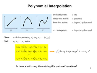
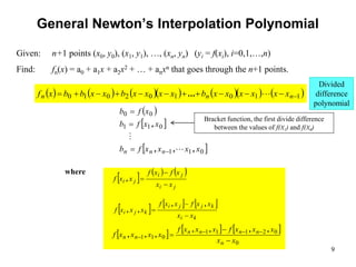
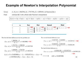
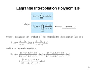
Given: three points (x0, y0), (x1, y1), (x2,y2)
Find: a quadratic f2(x) = a0 + a1x + a2x2 that goes through the three points.
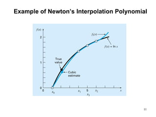
Example: f(x) = ln x
Data points:
b0 = 0
b1 = (1.386294 – 0)/(4 – 1) = 0.4620981
b2 = [(1.791759 – 1.386294)/(6-4) – 0.4620981]/(6-1)
= -0.0518731
f2(2) = 0.5658444
ln 2 = 0.6931472](https://image.slidesharecdn.com/appliednumericalmethodslec9-150507042342-lva1-app6892/85/Applied-numerical-methods-lec9-8-320.jpg)

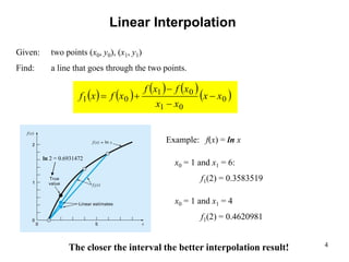
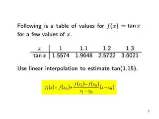
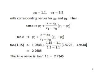
This document discusses various methods for polynomial interpolation of data points, including Newton's divided difference interpolating polynomials and Lagrange interpolation polynomials. It provides formulas and examples for linear, quadratic, and general polynomial interpolation using Newton's method. It also covers an example of using multiple linear regression with log-transformed data to develop a model relating fluid flow through a pipe to the pipe's diameter and slope.