Download as PDF, PPTX


![8
Finite-Difference Approach
(An Example)
2
11 2
x∆
+−
= −+
=
iii
xx
2
2
TTT
dx
Td
i
( ) 0h'
dx
d
a2
2
=−+ TT
T
( ) 0
2
2
11
=−
∆
+− −+
ai
iii
T-Th'
x
TTT
( ) aiii Txh'TTxh'T 2
1
2
1 2 ∆=−∆++− +−
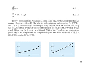
Instance: Ta =20, T(0) = 40, T(10) = 200, and h’ = 0.01; use ∆x = 2
=
−
−−
−−
−
8200
80
80
840
042100
104210
010421
001042
4
3
2
1
.
.
.
.
.
.
.
.
T
T
T
T
[ ] [ ]2004795159538212477859396986540543210 ....=TTTTTT
Centered finite difference](https://image.slidesharecdn.com/appliednumericalmethodslec14-150507042430-lva1-app6891/85/Applied-numerical-methods-lec14-8-320.jpg)
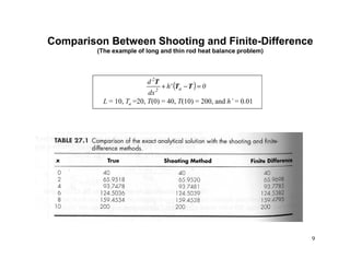
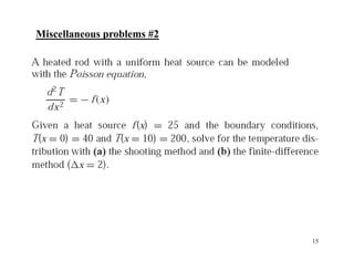
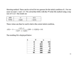
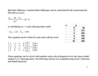
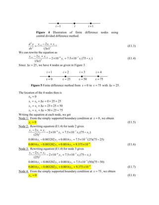

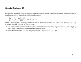

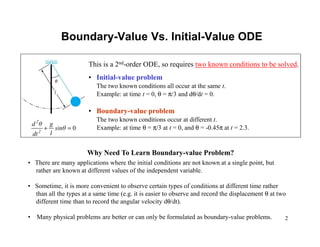
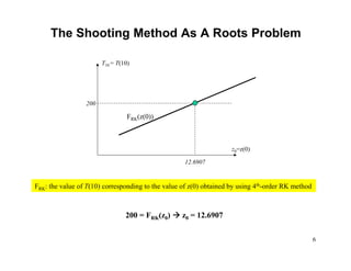
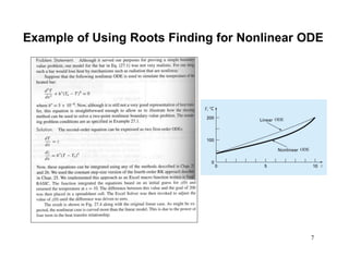
This document discusses boundary value problems and their solution using finite difference and shooting methods. It provides an example of using the finite difference method to solve a second order boundary value problem modeling heat transfer in a rod. The key steps are: 1) Discretizing the rod into nodes separated by a step size Δx and approximating derivatives as finite differences. 2) Setting up a system of equations relating the temperature at each node. 3) Solving the system of equations to find the temperature profile across the rod. 4) Calculating errors between the approximate and exact solutions. The shooting method is also discussed as an alternative approach, where the boundary value problem is converted to an initial value