The document discusses various techniques for fitting curves to data including linear regression, polynomial regression, and linearization of nonlinear relationships. Linear regression finds the line that best fits a set of data points by minimizing the sum of the squared residuals. The normal equations are derived and solved to determine the slope and intercept. Polynomial regression extends this to find the best-fit polynomial curve through the data. An example shows fitting a second-order polynomial. Nonlinear relationships can sometimes be linearized by a transformation of variables to apply linear regression. Examples demonstrate applying these techniques.

1. 1
Curve Fitting and Interpolation
Least-Squares Regression

2. 2
• Fit the best curve to a discrete data set and
obtain estimates for other data points
• Two general approaches:
– Data exhibit a significant degree of scatter
Find a single curve that represents the
general trend of the data.
– Data is very precise. Pass a curve(s)
exactly through each of the points.
• Two common applications in engineering:
Trend analysis. Predicting values of dependent
variable: extrapolation beyond data points or
interpolation between data points.
Hypothesis testing. Comparing existing
mathematical model with measured data.
Curve Fitting

3. 3
In sciences, if several measurements are made of a particular quantity,
additional insight can be gained by summarizing the data in one or more
well chosen statistics:
Arithmetic mean - The sum of the individual data points (yi)
divided by the number of points.
Standard deviation – a common measure of spread for a sample
or variance
Coefficient of variation –
quantifies the spread of data (similar to relative error)
n
i
n
y
y i
,
,
1 



1
2




n
y
y
S i
y
)
(
1
2
2




n
y
y
S i
y
)
(
Simple Statistics
%
100
.
.
y
S
v
c
y


4. 4
yi : measured value
e : error
yi = a0 + a1 xi + e
e = yi - a0 - a1 xi
a1 : slope
a0 : intercept
Linear Regression
e Error
Line equation
y = a0 + a1 x
Given: n points (x1, y1), (x2, y2), …, (xn, yn)
Find: a line y = a0 + a1x that best fits the n points.

5. 5
• Best strategy is to minimize the sum of the squares of the
residuals between the measured-y and the y calculated with the
linear model:
• Yields a unique line for a given set of data
• Need to compute a0 and a1 such that Sr is minimized!












n
i
i
i
r
n
i
model
i
measured
i
n
i
i
r
x
a
a
y
S
y
y
e
S
1
2
1
0
1
2
1
2
)
(
)
( ,
,
e Error
Minimize the sum of the residual errors for all available data?

6.   0
0
)
(
2
0
0
)
(
2
2
1
0
1
1
1
0
1






















 


 


i
i
i
i
i
i
o
i
r
i
i
i
o
i
o
r
x
a
x
a
x
y
x
x
a
a
y
a
S
x
a
a
y
x
a
a
y
a
S
Normal equations which can
be solved simultaneously
 
    i
i
i
i
i
i
x
y
a
x
a
x
y
a
x
na
na
a











1
2
0
1
0
0
0
(2)
(1)
Since

 





n
i
i
i
n
i
i
r x
a
a
y
e
S
1
2
1
0
1
2
)
(
:
error
Minimize
Least-Squares Fit of a Straight Line

7. 7
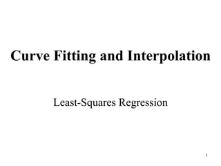
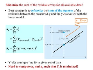
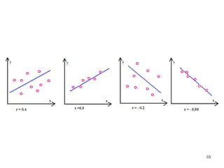
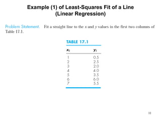
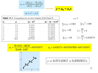
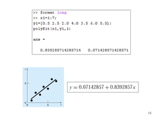
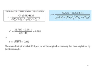
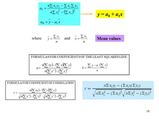
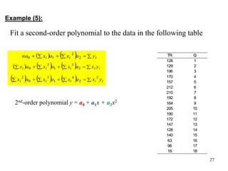
Least-Squares Fit of a Line
 
 






0
2 1
0
0
i
i
r
x
a
a
y
a
S
 
 






0
]
[
2 1
0
1
i
i
i
r
x
x
a
a
y
a
S
  


 i
i y
a
x
na 1
0
To minimize Sr:
where and
 
 

  

 2
2
1
i
i
i
i
i
i
x
x
n
y
x
y
x
n
a
    



 i
i
i
i y
x
a
x
a
x 1
2
0
x
a
y
a 1
0 

n
y
y i


n
x
x i


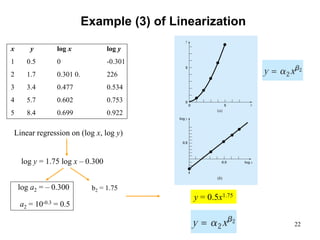
y = a0 + a1x
Mean values

8. 8
where and
 
 

  

 2
2
1
i
i
i
i
i
i
x
x
n
y
x
y
x
n
a
x
a
y
a 1
0 

n
y
y i


n
x
x i


y = a0 + a1x
Mean values

9. 9
Is our prediction reliable?
Once an equation is found for the least square line, we need to have
some way of judging just how good the equation is for predictive
purposes. In order to have a quantitative basis for confidence in our
predictions, we need to calculate coefficient of correlation, denoted
r. It may be calculated using the following formula:
The value of r that is close to 1 or -1 (r2 = 1 ) indicates that our
formula will give us a reliable prediction

10. 10

11. 11
Example (1) of Least-Squares Fit of a Line
(Linear Regression)

12. 12
7

n
5
119.

 i
i y
x 140
2

 i
x
  28
i
x 4
7
28


x
24

 i
y 428571
3
7
24
.


y
   
   
8392857
0
28
140
7
24
28
5
119
7
2
1 .
.




a   07142857
0
4
8392857
0
428571
3
0 .
.
. 


a
y = a0 + a1x

13. 13

14. 14

15. 15

16. 16

17. Example (2):
17
A sales manager noticed that the annual sales of his employees increase
with years of experience. To estimate the annual sales for his potential
new sales person he collected data concerning annual sales and years of
experience of his current employees: use his data to create a formula that
will help him estimate annual sales based on years of experience.

18. 18
where and
 
 

  

 2
2
1
i
i
i
i
i
i
x
x
n
y
x
y
x
n
a
x
a
y
a 1
0 

n
y
y i


n
x
x i


y = a0 + a1x
Mean values

19. 19

20. 20

21. 21
Linearization of Nonlinear Relationships
Nonlinear regression
Linear transformation (if possible)
Data that don’t fit linear form

22. 22
Example (3) of Linearization
Linear regression on (log x, log y)
b2 = 1.75
x y log x log y
1 0.5 0 -0.301
2 1.7 0.301 0. 226
3 3.4 0.477 0.534
4 5.7 0.602 0.753
5 8.4 0.699 0.922
log y = 1.75 log x – 0.300
log a2 = – 0.300
a2 = 10-0.3 = 0.5
y = 0.5x1.75

23. 23
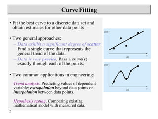
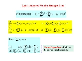
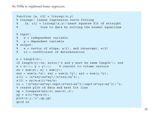
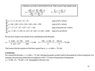
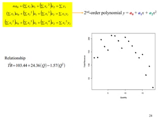
Polynomial Regression
)
1
( 


m
n
S
s r
x
y /
 
2
1
2
2
1
0
 






n
i
m
i
m
i
i
i
r x
a
x
a
x
a
a
y
S ...
 
2
1
2
2
1
0
 




n
i
i
i
i
r x
a
x
a
a
y
S
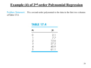
Given: n points (x1, y1), (x2, y2), …, (xn, yn)
Find: a polynomial y = a0 + a1x + a2x2 + … amxm that minimizes
Example: 2nd-order polynomial y = a0 + a1x + a2x2
 
 







0
2 2
2
1
0
0
i
i
i
r
x
a
x
a
a
y
a
S
 
 







0
]
[
2 2
2
1
0
1
i
i
i
i
r
x
x
a
x
a
a
y
a
S
 
 







0
]
[
2
2
2
2
1
0
2
i
i
i
i
r
x
x
a
x
a
a
y
a
S
    




 i
i
i y
a
x
a
x
na 2
2
1
0
      





 i
i
i
i
i y
x
a
x
a
x
a
x 2
3
1
2
0
      





 i
i
i
i
i y
x
a
x
a
x
a
x
2
2
4
1
3
0
2
Standard error:

24. 24
Example (4) of 2nd-order Polynomial Regression

25. 25
m = 2 ∑xi = 15 ∑xi
4 = 979
n = 6 ∑yi = 152.6 ∑xiyi = 585.6
∑xi
2= 55 ∑xi
2yi = 2488.9
∑xi
3= 225































8
2488
6
585
6
152
979
225
55
225
55
15
55
15
6
2
1
0
.
.
.
a
a
a
5
2.

x
y = 2.47857 + 2.35929x + 1.86071x2
12
1
3
6
74657
3
.
.
/ 


x
y
s 99851
0
39
2513
74657
3
39
2513
2
.
.
.
.





t
r
t
S
S
S
r
433
25.

y
    




 i
i
i y
a
x
a
x
na 2
2
1
0
      





 i
i
i
i
i y
x
a
x
a
x
a
x 2
3
1
2
0
      





 i
i
i
i
i y
x
a
x
a
x
a
x
2
2
4
1
3
0
2
2nd-order polynomial y = a0 + a1x + a2x2

26. 26
y = 2.47857 + 2.35929x + 1.86071x2

27. Example (5):
27
Fit a second-order polynomial to the data in the following table
    




 i
i
i y
a
x
a
x
na 2
2
1
0
      





 i
i
i
i
i y
x
a
x
a
x
a
x 2
3
1
2
0
      





 i
i
i
i
i y
x
a
x
a
x
a
x
2
2
4
1
3
0
2
2nd-order polynomial y = a0 + a1x + a2x2

28. 28
    




 i
i
i y
a
x
a
x
na 2
2
1
0
      





 i
i
i
i
i y
x
a
x
a
x
a
x 2
3
1
2
0
      





 i
i
i
i
i y
x
a
x
a
x
a
x
2
2
4
1
3
0
2
2nd-order polynomial y = a0 + a1x + a2x2

29. 29
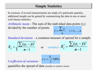
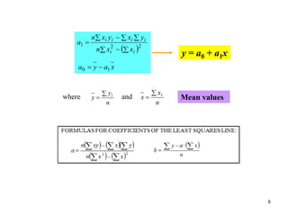
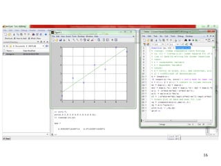
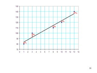
Multiple Linear Regression
 
 







0
]
[
2 2
2
2
1
1
0
2
i
i
i
i
r
x
x
a
x
a
a
y
a
S
 
2
1
2
2
1
1
0
 




n
i
i
i
i
r x
a
x
a
a
y
S
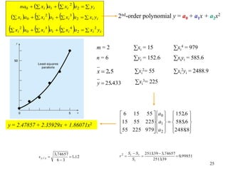
Given: n points 3D (y1, x11, x12) (y2, x12, x22), …, (yn, x1n, x2n)
Find: a plane y = a0 + a1x1 + a2x2 that minimizes
 
 







0
2 2
2
1
1
0
0
i
i
i
r
x
a
x
a
a
y
a
S
 
 







0
]
[
2 1
2
2
1
1
0
1
i
i
i
i
r
x
x
a
x
a
a
y
a
S
    




 i
i
i y
a
x
a
x
na 2
2
1
1
0
      





 i
i
i
i
i
i y
x
a
x
x
a
x
a
x 1
2
2
1
1
2
1
0
1
      





 i
i
i
i
i
i y
x
a
x
a
x
x
a
x 2
2
2
2
1
2
1
0
2
Generation to m dimensions:
hyper plane y = a0 + a1x1 + a2x2 + … + amxm

30. 30
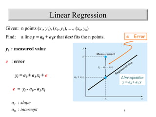
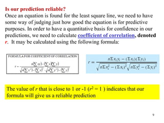
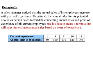
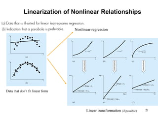
General Linear Least Squares


















































n
m
mn
n
n
m
m
n e
e
e
a
a
a
z
z
z
z
z
z
z
z
z
y
y
y










2
1
1
0
1
0
2
12
02
1
11
01
2
1
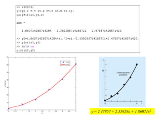
Linear least squares: y = a0 + a1x1
Multi-linear least squares: y = a0 + a1x1 + a2x2 + … + amxm
Polynomial least squares: y = a0 + a1x + a2x2 + … amxm
2
1 0
1
2
 












 

n
i
m
j
ji
j
i
n
i
i
r z
a
y
e
S
   
      
 
Y
Z
A
Z
Z
T
T

y = a0z0 + a1z1 + a2z2 + … + amzm
{Y} = [Z] {A} + {E}
[C] {A} = {D}
([C] is symmetric, e.g. linear and polynomial)