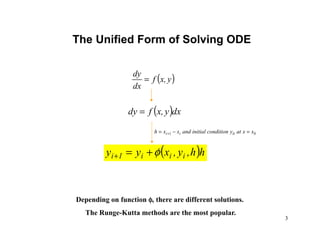
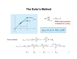
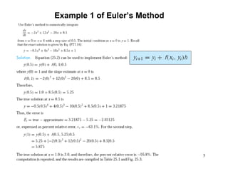
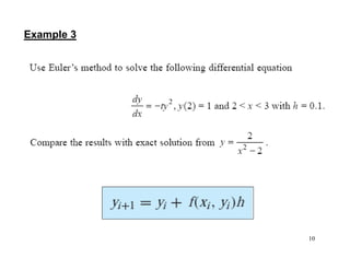
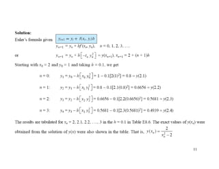
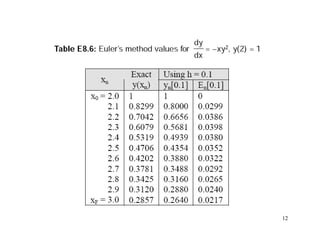
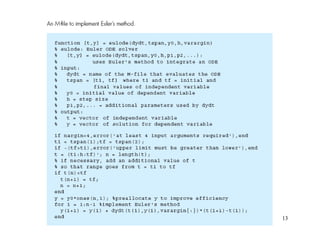
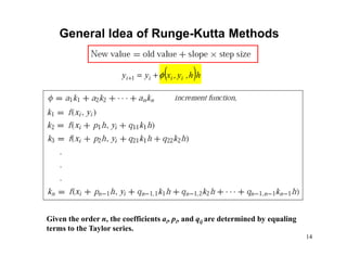
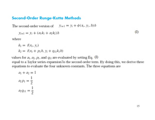
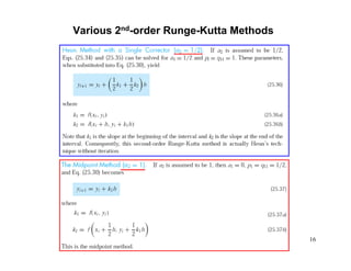
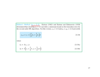
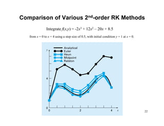
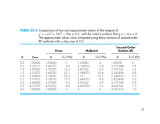
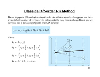
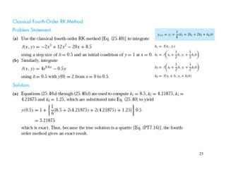
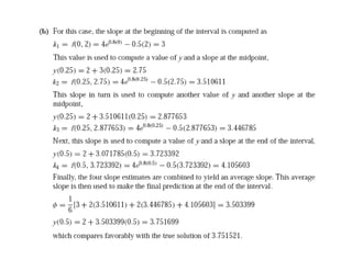
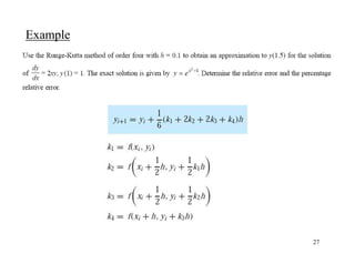
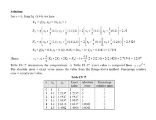
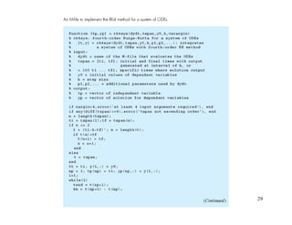
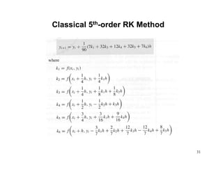
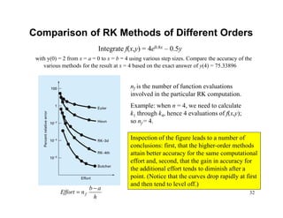
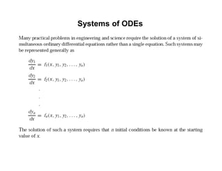
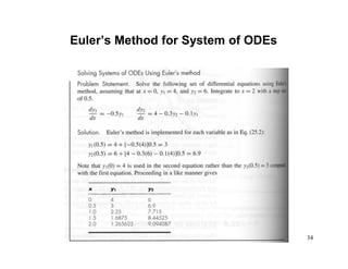
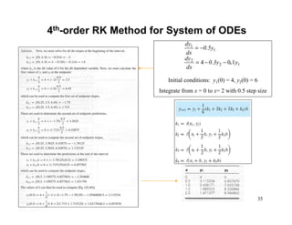
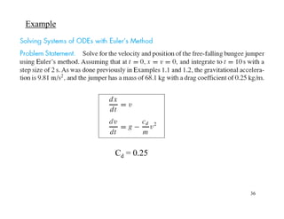
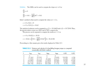
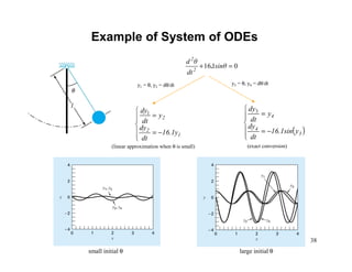
This document discusses numerical methods for solving ordinary differential equations (ODEs), including: 1) Initial-value problems where conditions are specified at a single value of the independent variable, unlike boundary-value problems. 2) Euler's method and higher-order Runge-Kutta methods for approximating solutions to ODEs using finite differences. Examples are provided to illustrate the methods. 3) Extensions of these methods to systems of ODEs, along with examples of applying the methods to coupled differential equations.

1. 1
Chapter 25ODE : Initial-value problem 1

2. 2
When dealing with an nth-order differential
equation, n conditions are required to obtain a
unique solution.
If all conditions are specified at the same value of
the independent variable (for example, at x or t = 0),
then the problem is called an initial-value problem.
This is in contrast to boundary-value problems
where specification of conditions occurs at different
values of the independent variable.

3. 3
The Unified Form of Solving ODE
( )dxyx,fdy =
( )hh,y,xyy iii1i φ+=+
Depending on function φφφφ, there are different solutions.
The Runge-Kutta methods are the most popular.
00ii xxatyconditioninitialandxxh =−= +1
( )yx,f
dx
dy
=

4. 4
The Euler’s Method
( )ii
xx
y,xf
dx
dy
i
==
=
φ
Error estimate:
( )
n
n
n
i2i
iii Rh
n!
y
h
2!
y
hyyy +++
′′
+′+=+ L1
( ) ( ) ( ) ( )( )
n
nii
1-n
3ii2ii
iiii Rh
n!
y,xf
h
3!
y,xf
h
2!
y,xf
hy,xfyy ++
′′
+
′
++=+ L1
Et = Et,2 + Et,3 + … + Et,n
Differential equation
evaluated at xi and yi

5. 5
Example 1 of Euler’s Method

6. 6

7. 7
Example 2

8. 8

9. 9
X0 =
y0 =
X1 =

10. Example 3
10

11. 11

12. 12

13. 13

14. 14
General Idea of Runge-Kutta Methods
Given the order n, the coefficients ai, pi, and qij are determined by equaling
terms to the Taylor series.
( )hh,y,xyy iiii φ+=+1

15. 15

16. 16
Various 2nd-order Runge-Kutta Methods

17. 17

18. 18
Example 4

19. 19

20. 20

21. 21

22. 22
Comparison of Various 2nd-order RK Methods
Integrate f(x,y) = -2x3 + 12x2 – 20x + 8.5
from x = 0 to x = 4 using a step size of 0.5, with initial condition y = 1 at x = 0.

23. 23

24. 24
Classical 4th-order RK Method

25. 25

26. 26

27. 27
Example

28. 28

29. 29

30. 30

31. 31
Classical 5th-order RK Method

32. 32
Comparison of RK Methods of Different Orders
Integrate f(x,y) = 4e0.8x – 0.5y
with y(0) = 2 from x = a = 0 to x = b = 4 using various step sizes. Compare the accuracy of the
various methods for the result at x = 4 based on the exact answer of y(4) = 75.33896
h
ab
nEffort f
−
=
nf is the number of function evaluations
involved in the particular RK computation.
Example: when n = 4, we need to calculate
k1 through k4, hence 4 evaluations of f(x,y);
so nf = 4.
Inspection of the figure leads to a number of
conclusions: first, that the higher-order methods
attain better accuracy for the same computational
effort and, second, that the gain in accuracy for
the additional effort tends to diminish after a
point. (Notice that the curves drop rapidly at first
and then tend to level off.)

33. Systems of ODEs

34. 34
Euler’s Method for System of ODEs

35. 35
4th-order RK Method for System of ODEs
12
2
1
1
104 y0.3y
dx
dy
0.5y
dx
dy
.−−=
−=
Initial conditions: y1(0) = 4, y2(0) = 6
Integrate from x = 0 to x= 2 with 0.5 step size

36. 36
Example
Cd = 0.25

37. 37

38. 38
Example of System of ODEs
( )





−=
=
3
4
4
y16.1sin
dt
dy
y
dt
dy3






−=
=
1
2
2
16.1y
dt
dy
y
dt
dy1
y1 = θ, y2 = dθ/dt
0116 =+ sinθ
dt
θd
2
2
.
(linear approximation when θ is small)
y3 = θ, y4 = dθ/dt
(exact conversion)
small initial θ large initial θ

39. 39
Special Problem 8

40. 40
Special Problem 9

41. Homework
41
1.
2.
3.
4.
5.

42. Homework
42
6.