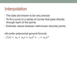
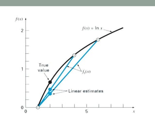
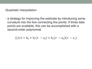
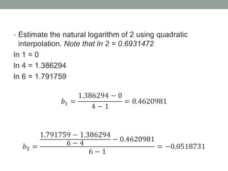
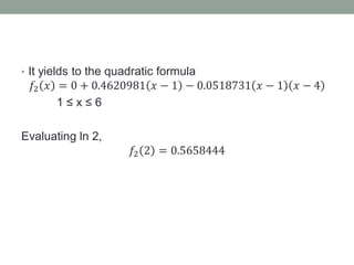
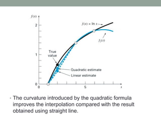
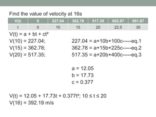
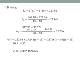
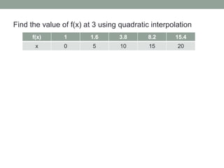
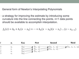
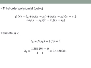
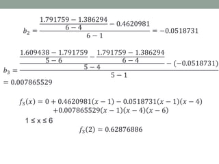
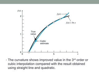
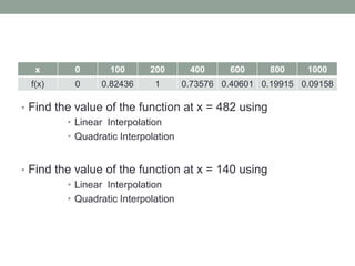
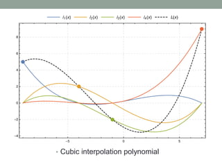
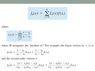
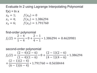
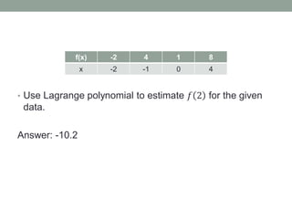
Interpolation
• The data are known to be very precise
• To fit a curve or a series of curves that pass directly
through each of the points.
• Estimate values between well-known discrete points.
nth-order polynomial general formula
• 𝑓 𝑥 = 𝑎0 + 𝑎1𝑥 + 𝑎2𝑥2
+ … + 𝑎𝑛𝑥𝑛
• Polynomial Interpolation
• consists of determining the unique nth-order polynomial that fits
n+1 data points. This polynomial then provides a formula to
compute intermediate values.
• Although there is one and only one nth-order polynomial that fits
n+1 points, there are a variety of mathematical formats in which
this polynomial can be expressed.
Polynomial Interpolation
• Newton’s Divided-Difference Interpolation Polynomials
• The simplest form of
interpolation is to connect
two data points with a
straight line. This technique,
called linear interpolation.
• Estimate the natural logarithm of 2 using linear
interpolation. Note that ln 2 = 0.6931472
• ln 1 = 0, ln 6 = 1.791759
𝑓1 2 = 0 +
1.791759 − 0
6 − 1
2 − 1 = 0.3583519
• ln 1 = 0, ln 4 = 1.386294
𝑓1 2 = 0 +
1.386294 − 0
4 − 1
2 − 1 = 0.4620981
V(t) 0 227.04 362.78 517.35 602.97 901.67
t 0 10 15 20 22.5 30
Find the value of velocity at 16s
V(t) = a + bt
V(15) = 362.78; 362.78 = a+15b-----eq.1
V(20) = 517.35; 517.35 = a+20b-----eq.2
a = -100.93
b = 30.914
V(t) = -100.93+30.914t; 15 ≤ t ≤ 20
V(16) = 393.7 m/s
• Similarly,
𝑉(16) = 362.78 +
517.35 − 362.78
20 − 15
16 − 15 = 393.694𝑚/𝑠
f(x) 1 1.6 3.8 8.2 15.4
x 0 5 10 15 20
Find the value of f(x) at 3.
• a strategy for improving the estimate by introducing some
curvature into the line connecting the points. If three data
points are available, this can be accomplished with a
second-order polynomial.
𝑓2 𝑥 = 𝑏0 + 𝑏1 𝑥 − 𝑥0 + 𝑏2(𝑥 − 𝑥0)(𝑥 − 𝑥1)
Quadratic Interpolation
• Estimate the natural logarithm of 2 using quadratic
interpolation. Note that ln 2 = 0.6931472
ln 1 = 0
ln 4 = 1.386294
ln 6 = 1.791759
𝑏1 =
1.386294 − 0
4 − 1
= 0.4620981
𝑏2 =
1.791759 − 1.386294
6 − 4
− 0.4620981
6 − 1
= −0.0518731
• It yields to the quadratic formula
𝑓2 𝑥 = 0 + 0.4620981 𝑥 − 1 − 0.0518731 𝑥 − 1 𝑥 − 4
1 ≤ x ≤ 6
Evaluating ln 2,
𝑓2 2 = 0.5658444
• The curvature introduced by the quadratic formula
improves the interpolation compared with the result
obtained using straight line.
V(t) 0 227.04 362.78 517.35 602.97 901.67
t 0 10 15 20 22.5 30
Find the value of velocity at 16s
V(t) = a + bt + ct²
V(10) = 227.04; 227.04 = a+10b+100c-----eq.1
V(15) = 362.78; 362.78 = a+15b+225c-----eq.2
V(20) = 517.35; 517.35 = a+20b+400c-----eq.3
a = 12.05
b = 17.73
c = 0.377
V(t) = 12.05 + 17.73t + 0.377t²; 10 ≤ t ≤ 20
V(16) = 392.19 m/s
• Similarly,
𝑏0 = 𝑓 𝑥0 = 𝑓(10) = 227.04
𝑏1 =
362.78 − 227.04
15 − 10
= 27.148
𝑏2 =
517.35 − 362.78
20 − 15
− 27.148
20 − 10
= 0.3766
𝑉 𝑡 = 227.04 + 27.148 𝑡 − 10 + 0.3766 𝑡 − 10 𝑡 − 15
10 ≤ t ≤ 20
V(16) = 392.1876m/s
f(x) 1 1.6 3.8 8.2 15.4
x 0 5 10 15 20
Find the value of f(x) at 3 using quadratic interpolation
• a strategy for improving the estimate by introducing some
curvature into the line connecting the points. n+1 data points
should be available to accomplish interpolation.
𝑓𝑛 𝑥 = 𝑏0 + 𝑏1 𝑥 − 𝑥0 + ⋯ + 𝑏𝑛 𝑥 − 𝑥0 𝑥 − 𝑥1 … (𝑥 − 𝑥𝑛−1)
General form of Newton’s Interpolating Polynomials
• Third order polynomial (cubic)
𝑓3 𝑥 = 𝑏0 + 𝑏1 𝑥 − 𝑥0 + 𝑏2 𝑥 − 𝑥0 𝑥 − 𝑥1
+𝑏3 𝑥 − 𝑥0 𝑥 − 𝑥1 (𝑥 − 𝑥2)
Estimate ln 2
𝑏0 = 𝑓 𝑥0 = 𝑓 0 = 0
𝑏1 =
1.386294 − 0
4 − 1
= 0.4620981
𝑏2 =
1.791759 − 1.386294
6 − 4 − 0.4620981
6 − 1
= −0.0518731
𝑏3 =
1.609438 − 1.791759
5 − 6
−
1.791759 − 1.386294
6 − 4
5 − 4
− (−0.0518731)
5 − 1
= 0.007865529
𝑓3 𝑥 = 0 + 0.4620981 𝑥 − 1 − 0.0518731 𝑥 − 1 𝑥 − 4
+0.007865529 𝑥 − 1 𝑥 − 4 𝑥 − 6
1 ≤ x ≤ 6
𝑓3 2 = 0.62876886
• The curvature shows improved value in the 3rd order or
cubic interpolation compared with the result obtained
using straight line and quadratic.
x 0 100 200 400 600 800 1000
f(x) 0 0.82436 1 0.73576 0.40601 0.19915 0.09158
• Find the value of the function at x = 482 using
• Linear Interpolation
• Quadratic Interpolation
• Find the value of the function at x = 140 using
• Linear Interpolation
• Quadratic Interpolation
• a reformulation of the Newton polynomial that avoids the
computation of divided differences.
• for a given set of points 𝑥𝑗, 𝑦𝑗 with no two 𝑥𝑗 values
equal, the Lagrange polynomial is the polynomial of the
lowest degree that assumes at each value 𝑥𝑗 the
corresponding value 𝑦𝑗, so that the functions coincide at
each point.
Lagrange Interpolating Polynomials
• Cubic interpolation polynomial
Example
Example
Evaluate ln 2 using Lagrange Interpolating Polynomial
f(x) = ln x
𝑥0 = 1; 𝑓 𝑥0 = 0
𝑥1 = 4; 𝑓 𝑥1 = 1.386294
𝑥2 = 6; 𝑓 𝑥2 = 1.791760
first-order polynomial
𝑓1 2 =
2 − 4
1 − 4
∗ 0 +
2 − 1
4 − 1
∗ 1.386294 = 0.4620981
second-order polynomial
𝑓2 2 =
2 − 4 2 − 6
1 − 4 1 − 6
∗ 0 +
2 − 1 2 − 6
4 − 1 4 − 6
∗ 1.386294
+
2 − 1 2 − 4
6 − 1 6 − 4
∗ 1.791760 = 0.5658444
• Use Lagrange polynomial to estimate 𝑓 2 for the given
data.
Answer: -10.2
f(x) -2 4 1 8
x -2 -1 0 4

Interpolation(2) Numerical methods to CE Problems).pdf

  • 1.
    Interpolation • The dataare known to be very precise • To fit a curve or a series of curves that pass directly through each of the points. • Estimate values between well-known discrete points. nth-order polynomial general formula • 𝑓 𝑥 = 𝑎0 + 𝑎1𝑥 + 𝑎2𝑥2 + … + 𝑎𝑛𝑥𝑛
  • 2.
    • Polynomial Interpolation •consists of determining the unique nth-order polynomial that fits n+1 data points. This polynomial then provides a formula to compute intermediate values. • Although there is one and only one nth-order polynomial that fits n+1 points, there are a variety of mathematical formats in which this polynomial can be expressed.
  • 3.
    Polynomial Interpolation • Newton’sDivided-Difference Interpolation Polynomials • The simplest form of interpolation is to connect two data points with a straight line. This technique, called linear interpolation.
  • 4.
    • Estimate thenatural logarithm of 2 using linear interpolation. Note that ln 2 = 0.6931472 • ln 1 = 0, ln 6 = 1.791759 𝑓1 2 = 0 + 1.791759 − 0 6 − 1 2 − 1 = 0.3583519 • ln 1 = 0, ln 4 = 1.386294 𝑓1 2 = 0 + 1.386294 − 0 4 − 1 2 − 1 = 0.4620981
  • 6.
    V(t) 0 227.04362.78 517.35 602.97 901.67 t 0 10 15 20 22.5 30 Find the value of velocity at 16s V(t) = a + bt V(15) = 362.78; 362.78 = a+15b-----eq.1 V(20) = 517.35; 517.35 = a+20b-----eq.2 a = -100.93 b = 30.914 V(t) = -100.93+30.914t; 15 ≤ t ≤ 20 V(16) = 393.7 m/s
  • 7.
    • Similarly, 𝑉(16) =362.78 + 517.35 − 362.78 20 − 15 16 − 15 = 393.694𝑚/𝑠
  • 8.
    f(x) 1 1.63.8 8.2 15.4 x 0 5 10 15 20 Find the value of f(x) at 3.
  • 9.
    • a strategyfor improving the estimate by introducing some curvature into the line connecting the points. If three data points are available, this can be accomplished with a second-order polynomial. 𝑓2 𝑥 = 𝑏0 + 𝑏1 𝑥 − 𝑥0 + 𝑏2(𝑥 − 𝑥0)(𝑥 − 𝑥1) Quadratic Interpolation
  • 10.
    • Estimate thenatural logarithm of 2 using quadratic interpolation. Note that ln 2 = 0.6931472 ln 1 = 0 ln 4 = 1.386294 ln 6 = 1.791759 𝑏1 = 1.386294 − 0 4 − 1 = 0.4620981 𝑏2 = 1.791759 − 1.386294 6 − 4 − 0.4620981 6 − 1 = −0.0518731
  • 11.
    • It yieldsto the quadratic formula 𝑓2 𝑥 = 0 + 0.4620981 𝑥 − 1 − 0.0518731 𝑥 − 1 𝑥 − 4 1 ≤ x ≤ 6 Evaluating ln 2, 𝑓2 2 = 0.5658444
  • 12.
    • The curvatureintroduced by the quadratic formula improves the interpolation compared with the result obtained using straight line.
  • 13.
    V(t) 0 227.04362.78 517.35 602.97 901.67 t 0 10 15 20 22.5 30 Find the value of velocity at 16s V(t) = a + bt + ct² V(10) = 227.04; 227.04 = a+10b+100c-----eq.1 V(15) = 362.78; 362.78 = a+15b+225c-----eq.2 V(20) = 517.35; 517.35 = a+20b+400c-----eq.3 a = 12.05 b = 17.73 c = 0.377 V(t) = 12.05 + 17.73t + 0.377t²; 10 ≤ t ≤ 20 V(16) = 392.19 m/s
  • 14.
    • Similarly, 𝑏0 =𝑓 𝑥0 = 𝑓(10) = 227.04 𝑏1 = 362.78 − 227.04 15 − 10 = 27.148 𝑏2 = 517.35 − 362.78 20 − 15 − 27.148 20 − 10 = 0.3766 𝑉 𝑡 = 227.04 + 27.148 𝑡 − 10 + 0.3766 𝑡 − 10 𝑡 − 15 10 ≤ t ≤ 20 V(16) = 392.1876m/s
  • 15.
    f(x) 1 1.63.8 8.2 15.4 x 0 5 10 15 20 Find the value of f(x) at 3 using quadratic interpolation
  • 16.
    • a strategyfor improving the estimate by introducing some curvature into the line connecting the points. n+1 data points should be available to accomplish interpolation. 𝑓𝑛 𝑥 = 𝑏0 + 𝑏1 𝑥 − 𝑥0 + ⋯ + 𝑏𝑛 𝑥 − 𝑥0 𝑥 − 𝑥1 … (𝑥 − 𝑥𝑛−1) General form of Newton’s Interpolating Polynomials
  • 17.
    • Third orderpolynomial (cubic) 𝑓3 𝑥 = 𝑏0 + 𝑏1 𝑥 − 𝑥0 + 𝑏2 𝑥 − 𝑥0 𝑥 − 𝑥1 +𝑏3 𝑥 − 𝑥0 𝑥 − 𝑥1 (𝑥 − 𝑥2) Estimate ln 2 𝑏0 = 𝑓 𝑥0 = 𝑓 0 = 0 𝑏1 = 1.386294 − 0 4 − 1 = 0.4620981
  • 18.
    𝑏2 = 1.791759 −1.386294 6 − 4 − 0.4620981 6 − 1 = −0.0518731 𝑏3 = 1.609438 − 1.791759 5 − 6 − 1.791759 − 1.386294 6 − 4 5 − 4 − (−0.0518731) 5 − 1 = 0.007865529 𝑓3 𝑥 = 0 + 0.4620981 𝑥 − 1 − 0.0518731 𝑥 − 1 𝑥 − 4 +0.007865529 𝑥 − 1 𝑥 − 4 𝑥 − 6 1 ≤ x ≤ 6 𝑓3 2 = 0.62876886
  • 19.
    • The curvatureshows improved value in the 3rd order or cubic interpolation compared with the result obtained using straight line and quadratic.
  • 20.
    x 0 100200 400 600 800 1000 f(x) 0 0.82436 1 0.73576 0.40601 0.19915 0.09158 • Find the value of the function at x = 482 using • Linear Interpolation • Quadratic Interpolation • Find the value of the function at x = 140 using • Linear Interpolation • Quadratic Interpolation
  • 21.
    • a reformulationof the Newton polynomial that avoids the computation of divided differences. • for a given set of points 𝑥𝑗, 𝑦𝑗 with no two 𝑥𝑗 values equal, the Lagrange polynomial is the polynomial of the lowest degree that assumes at each value 𝑥𝑗 the corresponding value 𝑦𝑗, so that the functions coincide at each point. Lagrange Interpolating Polynomials
  • 22.
  • 24.
  • 25.
  • 26.
    Evaluate ln 2using Lagrange Interpolating Polynomial f(x) = ln x 𝑥0 = 1; 𝑓 𝑥0 = 0 𝑥1 = 4; 𝑓 𝑥1 = 1.386294 𝑥2 = 6; 𝑓 𝑥2 = 1.791760 first-order polynomial 𝑓1 2 = 2 − 4 1 − 4 ∗ 0 + 2 − 1 4 − 1 ∗ 1.386294 = 0.4620981 second-order polynomial 𝑓2 2 = 2 − 4 2 − 6 1 − 4 1 − 6 ∗ 0 + 2 − 1 2 − 6 4 − 1 4 − 6 ∗ 1.386294 + 2 − 1 2 − 4 6 − 1 6 − 4 ∗ 1.791760 = 0.5658444
  • 27.
    • Use Lagrangepolynomial to estimate 𝑓 2 for the given data. Answer: -10.2 f(x) -2 4 1 8 x -2 -1 0 4