Downloaded 10 times


![Introduction
Say that, in the study of some phenomenon, there is an established functional
relationship between the quantities y and x; but the function f(x) is unknown.
The experiment has established the values of the function y0, y1, . . . , yN for cer-
tain values of the argument x0, x1, . . . , xN in the interval [x0, xN ]. We don't
have an analytic expression for f(x). The problem is then to nd a function (as
simple as possible from the computational stand-point; for example a polyno-
mial) which will represent the unknown function y = f(x).
In more abstract fashion, the problem may be formulated as follows: given on
the interval [x0, xN ], the values of an unknown function y = f(x) at N + 1
distinct points x0, x1, . . . , xN , such that,
y0 = f(x0), y1 = f(x1), . . . , yN = f(xN )
It is required to nd a polynomial P(x) of degree≤ n that approximately
expresses the function f(x). Further, the task is to estimate f(x) for some
target value of x.
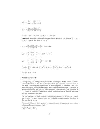
Interpolating polynomial given one data point and
its higher order derivatives
Say that, we are required to t a polynomial P(x), at a point x = x0, where
the value of the function and the value of its rst n derivatives at that point
f(x0), f (x), f(2)
(x), . . . , f(n)
(x) are given. Then, the Taylor's series expansion
of the function in terms of a polynomial of degree n over the interval [x0, x] is
the interpolating polynomial. This is intuitive, because the Taylor's series
polynomial and its higher order derivatives have the same values as the function
and its derivatives.
The Taylor's series expansion of a function f(x) over the interval [x0, x], such
that Pn(x0) = f(x0), Pn(x0) = f (x0), Pn (x0) = f (x0), . . . , P
(n)
n (x0) = f(n)
(x0)
is given as
Pn(x) = f(x0) + (x−x0)
1! f (x0) + (x−x0)2
2! f (x0) + . . . + (x−x0)n
n! f(n)
(x) + Rn(x)
Rn(x) is called the remainder. For those values of x, for which the Rn(x) is small,
the polynomial Pn(x) yields an approximate representation of the function f(x).
On interpolating any value using the polynomial Pn(x), it is necessary to know,
the degree of accuracy of the estimate, or the error. The remainder term can
be expressed in the form
Rn(x) = (x−x0)(n+1)
(n+1)! f(n+1)
(ξ), where x0 ξ x
1](https://image.slidesharecdn.com/interpolationnotes-160727120655/85/Interpolation-techniques-Background-and-implementation-2-320.jpg)
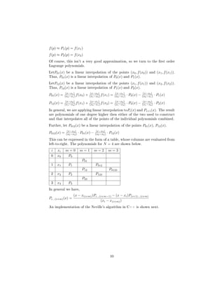
![Error term
The error in an interpolation is of prime importance. For example, we may be
given N = 1000 data points. To construct an interpolating polynomial, we may
use only M = 4 points. What will be the error in that approximation. Further,
is there an upper bound on the error - what is the largest possible error in that
interpolation. The answers to these questions will be known through the error
term.
We have,
Rn(x) =
1
(n + 1)!
· |(x − x0)|n+1
· |fn+1
(ξ)|
≤
1
(n + 1)!
· |(x − x0)|n+1
· Mn+1
where Mn+1 is the maximum value of fn+1
(ξ) over an interval [x0, x].
Assume that an estimate of Mn+1is available. Suppose, we are asked to con-
struct a 5-term Taylor's series. Say, we desire have an error no more than an
acceptable tolerance, that is|Rn(x)| . To fulll this condition, we must have,
|Rn(x)| = 1
(n+1)! · |(x − x0)|n+1
· Mn+1
Conclusions:
1. If the tolerance and the number of terms in the Taylor's series n are given
to us, then we can easily nd out the distance h from the point x0, so that the
accuracy is retained.
2](https://image.slidesharecdn.com/interpolationnotes-160727120655/85/Interpolation-techniques-Background-and-implementation-3-320.jpg)
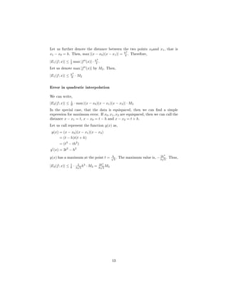
![2. If the distance h and the tolerance are given, we can solve for n, the number
of terms required in the Taylor's series, so that the accuracy is retained.
Example. Obtain the polynomial approximation to f(x) =
√
1 + x over the
interval [0, 1] by means of Taylor's series, about the point x0 = 0.
(i) Estimate the error of the approximate equation
√
1 + x ≈ 1+ 1
2 x− 1
8 x2
when
x = 0.2.
(ii) Find the number of terms required in the expansion to obtain results correct
to 5 × 10⁻⁶
for 0 x 1
2 .
Solution.
i f(i)
(x) f(i)
(0)
0 (1 + x)1/2
1
1 1
2 (1 + x)−1/2 1
2
2 − 1
22 (1 + x)−3/2
− 1
22
3 1·3
23 (1 + x)−5/2 1·3
23
n (−1)n−1
· 1·3·...·(2n−3)
2n (1 + x)−(2n−1)/2
(−1)n 1·3·...·(2n−3)
2n
n + 1 (−1)n
· 1·3·...·(2n−1)
2n+1 (1 + x)−(2n+1)/2
Therefore, our polynomial approximation is,
P(x) = 1 +
1
2
x −
1
2!
1
22
x2
+
1
3!
1 · 3
23
x3
+ . . . +
(−1)n−1
xn
n!
·
1 · 3 · . . . · (2n − 3)
2n
+ Rn(x)
= 1 +
x
2
−
x2
8
+
x3
16
+ . . . +
(−1)n−1
xn
n!
·
1 · 3 · . . . · (2n − 3)
2n
+ Rn(x)
(i) The maximum of f(n+1)
(x) in the interval [0, 1
2 ] is as follows.
f(n+1)
(x) = 1·3·...·(2n−1)
2n+1 · 1
(1+x)(2n+1)/2
This will be maximum when (1 + x) is minimum, or x is minimum. Thus,
f(n+1)
(x) will be maximum at x = 0.
Mn+1 = 1·3·...·(2n−1)
2n+1 = (2n)!
2nn! · 1
2n+1 = 1
22n+1 · (2n)!
n!
Rn(x) ≤ 1
(n+1)! · |x|n
· Mn+1 = 1
(n+1)! · |x|n+1
· 1
22n+1 · (2n)!
n!
At x = 0.2, n = 2,
3](https://image.slidesharecdn.com/interpolationnotes-160727120655/85/Interpolation-techniques-Background-and-implementation-4-320.jpg)
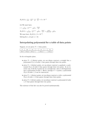
![Program listing. Neville's method
/∗ Polynomial interpolation f i t t i n g a set of data points
xx [ 0 . . . n−1], yy [ 0 . . . n−1]. This r e s u l t s in a polynomial
approximation of order (n−1). ∗/
void poly_interp ( f l o a t ∗xx , f l o a t ∗yy , f l o a t x , i n t n , f l o a t ∗y) {
f l o a t ∗P = new f l o a t [ n ] ;
i n t m, i ;
f o r (m = 0; m n ; m++) {
f o r ( i = 0; i n − m; i++) {
i f (m 0) {
P[ i ] = (( x − xx [ i + m])∗ (P[ i ] ) −
(x − xx [ i ])∗ (P[ i + 1])) / (xx [ i ] − xx [ i + m] ) ;
}
e l s e {
P[ i ] = yy [ i ] ;
}
}
}
∗y = P[ 0 ] ;
}
Error of interpolation
Let us denote the error of interpolation as,
En(f; x) = f(x) − Pn(x)
We are also given the N + 1 data points.
x x0 x1 . . . xi . . . xn
f(x) f(x0) f(x1) . . . f(xi) . . . f(xn)
Since, the interpolating polynomial ts the above data points, there is no error
at the nodal points.
En(f; xi) = f(xi) − P(xi) = 0
Let us denote the rst point x0 = a and the last point xn = b. Let us choose
an arbitrary point x at which we are interpolating f(x). Therefore, x ∈ [a, b].
Let us dene an auxiliary function,
g(t) = [f(t) − P(t)] − [f(x) − P(x)] (t−x0)(t−x1)...(t−xn)
(x−x0)(x−x1)...(x−xn)
g(t) is a continuous function.
11](https://image.slidesharecdn.com/interpolationnotes-160727120655/85/Interpolation-techniques-Background-and-implementation-12-320.jpg)
![(i) At t = x,g(x) = 0.
(ii) At t = xi, g(xi) = f(xi) − P(xi) = 0
Thus, the function g(t) vanishes at N + 2 points, x0, x1, x2, . . . , xn. Also, g(t)
is dierentiable on each of the sub-intervals [x0, x1], [x1, x2], . . . , [xn−1, xn].
Applying Rolle's theorem, there must be atleast one point c1, c2, . . . , ci, . . . , cn
in each of these sub-intervals such that g (ci) = 0.
Now, if we apply Rolle's theorem to the function g (t) over the sub-intervals
[c1, c2], [c2, c3], . . . , [cn−1, cn], then there exist points di : i = 1, 2, . . . , n − 1 in
each of these sub-intervals where the second derivative g (t) = 0.
Continuing in this fashion and applying Rolle's theorem iteratively n + 1 times
(since there are N + 2 points), there must be atleast one point in the interval
ξ ∈ [x0, xn], such that g(n+1)
(ξ) = 0.
Let us now dierentiate g(t), n + 1 times. Note that P(t) is a polynomial of
degree n. Hence, its (n + 1)'th derivative is zero.
g(n+1)
(ξ) = f(n+1)
(ξ) − 0 − [f(x)−P (x)](n+1)!
(x−x0)(x−x1)...(x−xn)
But, g(n+1)
(ξ) = 0.
Therefore, En(f; x) = f(x) − P(x) = f(n+1)
(ξ) · w(x)
(n+1)!
The magnitude of f(x) − P(x), would be:
|f(x) − P(x)| = 1
(n+1)! · |w(x)| · |f(n+1)
(ξ)|
Since ξ is unknown to us, we don't know, what is the exact value of f(n+1)
(ξ)
is. But, we can establish an upper bound on the error. We take the maximum
possible value of f(n+1)
(x). Therefore,
|f(x) − P(x)| ≤ 1
(n+1)! · max |w(x)| · max |f(n+1)
(x)|
Error in linear interpolation
We can express E1(f; x) as,
E1(f; x) = f (ξ) · (x−x0)(x−x1)
2!
|E1(f; x)| ≤ 1
2 max |f (x)| · max |(x − x0)(x − x1)|
The maximum of the expression (x − x0)(x − x1) is found by setting the rst
derivative to zero.
h(x) = x2
− (x0 + x1)x + x0x1
h (x) = 2x − (x0 + x1)
The function h(x) has a maximum at x = x0+x1
2 . The maximum value of h(x)
is, h x0+x1
2 = x1
2 − x0
2
x0
2 − x1
2 = −(x1−x0)2
4 .
12](https://image.slidesharecdn.com/interpolationnotes-160727120655/85/Interpolation-techniques-Background-and-implementation-13-320.jpg)

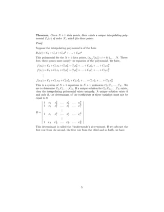
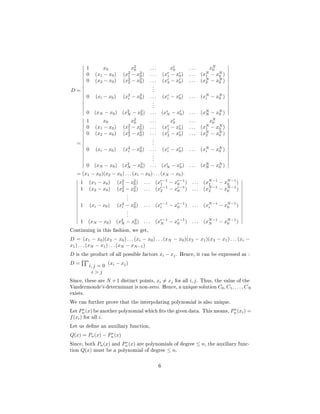
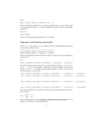
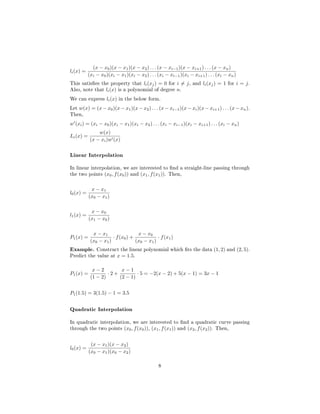
This document discusses interpolation techniques, specifically Lagrange interpolation. It begins by introducing the problem of interpolation - given values of an unknown function f(x) at discrete points, finding a simple function that approximates f(x). It then discusses using Taylor series polynomials for interpolation when the function value and its derivatives are known at a point. The error in interpolation approximations is also examined. The main part discusses Lagrange interpolation - given data points (xi, f(xi)), there exists a unique interpolating polynomial Pn(x) of degree N that passes through all the points. This is proved using the non-zero Vandermonde determinant. Lagrange's interpolating polynomial is then introduced as a solution.