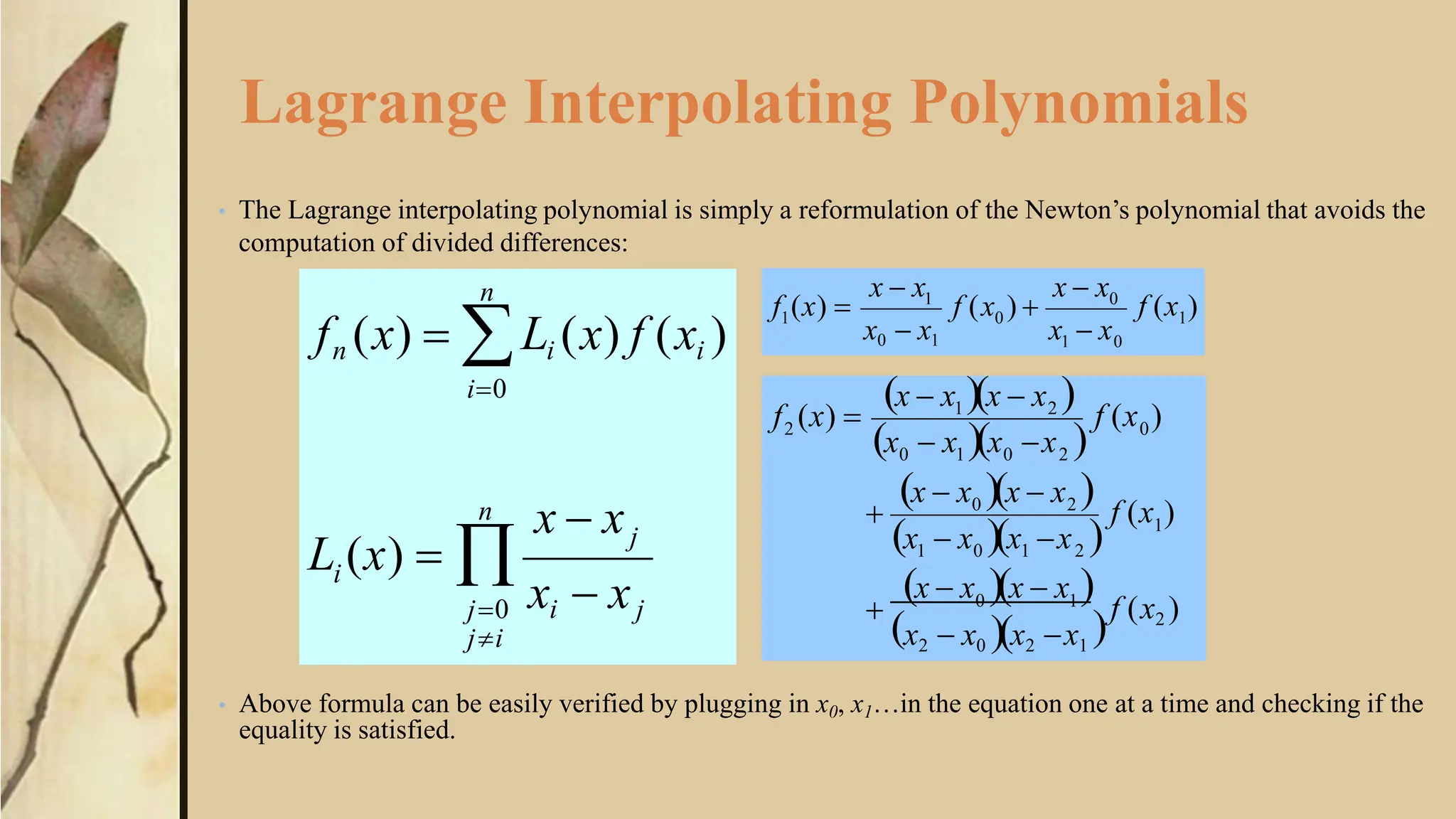
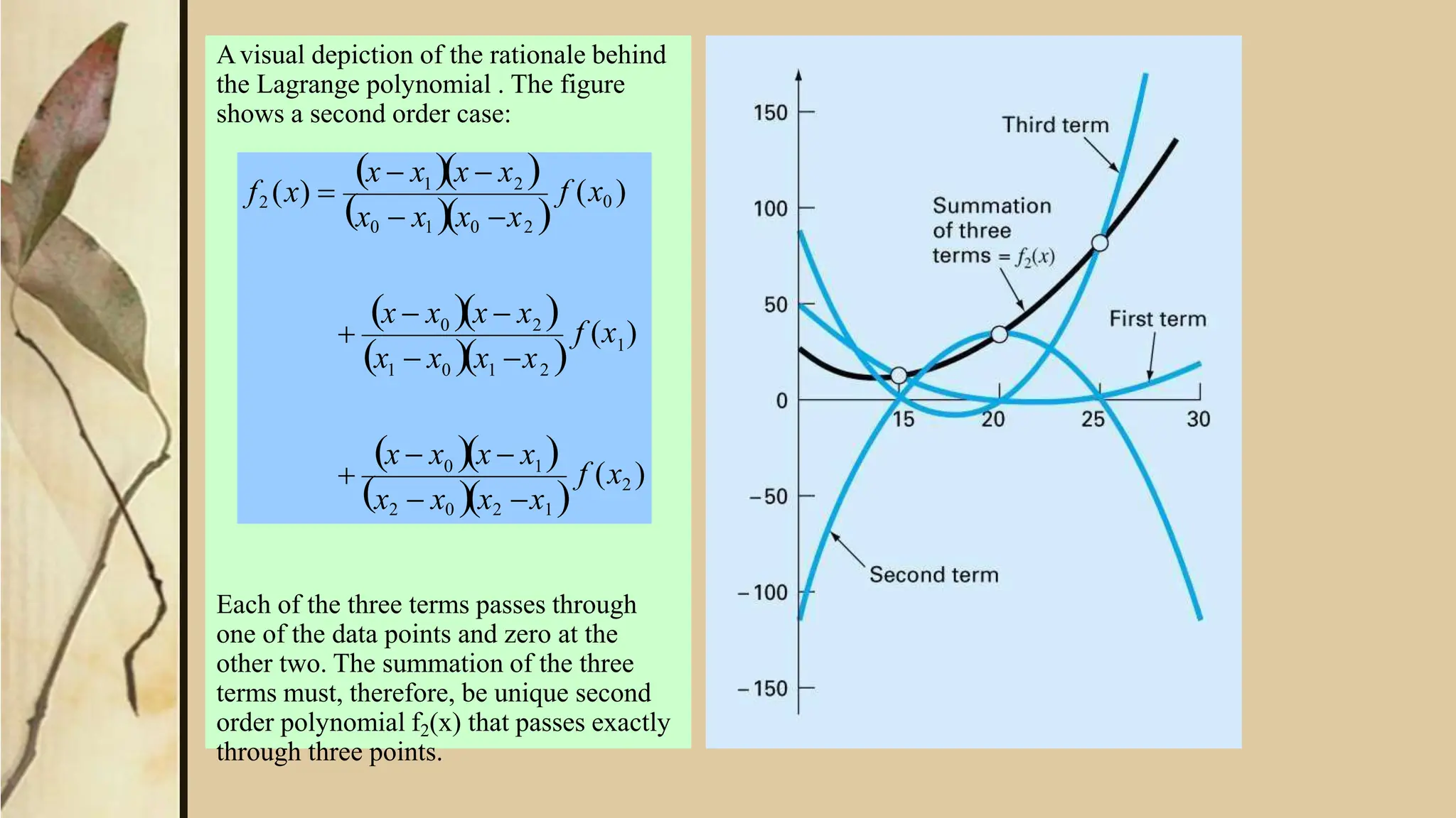
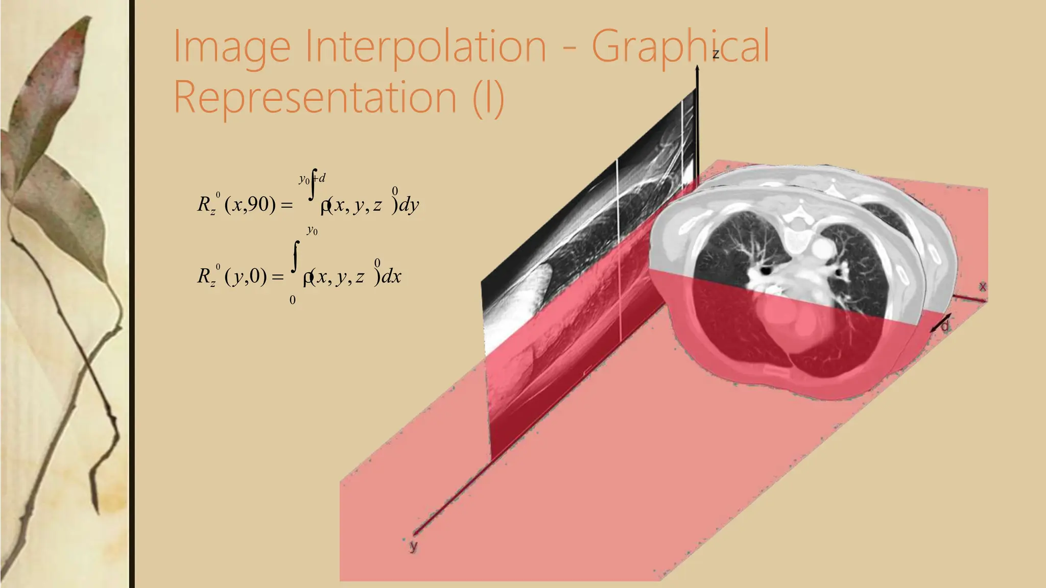
This document discusses different methods of interpolation, including Newton's divided-difference interpolating polynomials and Lagrange interpolating polynomials. Newton's method uses finite divided differences to determine the coefficients of a polynomial that fits a set of data points exactly. Lagrange's method expresses the interpolating polynomial as a weighted sum of basis polynomials, where each basis polynomial passes through one data point. The document also provides an example of using Newton's method to interpolate logarithm values and estimates the logarithm of 2. Image interpolation techniques like Radon reconstruction are discussed, which reconstruct an image from its projections by approximating the inverse Radon transform.

1. T
opic:-
Interpolation
B.S.N.V. PG COLLEGE CHARBAGH , LUCKNOW
Name- Akhil Kumar Singh
Roll No-2110084010029
Class – Bsc-5th semester

2. Contents
⚫Introduction
⚫Newton’s Divided-Difference Interpolating Polynomials
⚫Error Estimation in Newton’s Interpolating
Polynomials
⚫Lagrange Interpolating Polynomials
⚫Image Interpolation - Theory

3. Introduction
Interpolation : Estimation of a function value at an intermediate point
that lie between precise data points.
⚫ There is one and only one nth-order polynomial that perfectly fits n+1 data points:
⚫ There are several methods to find the fitting polynomial:
the Newton polynomial and the Lagrange polynomial (unequal
interval)

4. Newton’s Divided-Difference Interpolating
Polynomials
f1(x) designates a first-order interpolating polynomial.
Linear Interpolation
Connecting two data points with a straight line
f1(x)  f (x0 )

f (x1)  f (x0 )
x  x0 x1  x0
Linear-
interpolation
formula
Slope
0
0
1
x  x
f (x1)  f (x0 )
f1(x)  f (x0 )  (x  x )

5. Quadratic Interpolation
• If three (3) data points are available, the estimate is improved by introducing some curvature into the line
connecting the points.
A second-order polynomial (parabola) can be used for this purpose
• A simple procedure can be used to determine the values of the coefficients
f2 (x)  b0  b1(x  x0 )  b2 (x  x0 )(x  x1)
x  x0 b0  f (x0 ) Could you
figure out how
to derive this
using the above
equation?
Represents a
second order
polynomial
f (x1)  f (x0 )
x  x1 b1 
2 0
2
2
x  x
x2  x1 x1  x0
b 
x  x
x1  x0
f (x2 )  f (x1)

f (x1)  f (x0 )

6. f (x)  b0  b1(x  x0 )  b2 (x  x0 )(x  x1)
2 0
2 0
1 0
(x  x )
x  x
f (x1)  f (x0 )
f (x )  f (x ) 
b2  1 0
(x2  x0 )(x2  x1) (x2  x0 )(x2  x1)
f (x )  f (x ) b (x  x )
b2  2 0 1 2 0
x  x2
x  x
f (x1)  f (x0 )
b0  f (x0 ) b1 
2
( f (x2 )  f (x1 ))(x2  x1 )

( f (x1 )  f (x0 ))(x2  x1 )
(x2  x1 ) (x1  x0 )
b 
2
(x2  x0 )
(x2  x1 ) (x1  x0 )
(x2  x0 )(x2  x1 )
f (x2 )  f (x1 )

f (x1 )  f (x0 )
b 
1 0
0 1 0
1
0 2 1
1
2 1
(x2  x0 )(x2  x1)
(x  x )
)  ( f (x )  f (x ))(x  x )
))(x  x
( f (x )  f (x
 ( f (x1)  f (x0 ))
(x  x )
( f (x2 )  f (x1))(x2  x1)
b2 
2 0 2 1
2
2
(x  x )(x  x )
( f (x2 )  f (x1)  f (x1)  f (x0 ))(x2  x1)

( f (x1)  f (x0 ))(x2  x1  x1  x0 )
(x2  x1) (x1  x0 )
b 
x  x

7. General Form of Newton’s Interpolating
Polynomials
xi  xj
f (xi ) f (xj )
f [xi , xj ] 
Bracketed function
evaluations are finite
divided differences
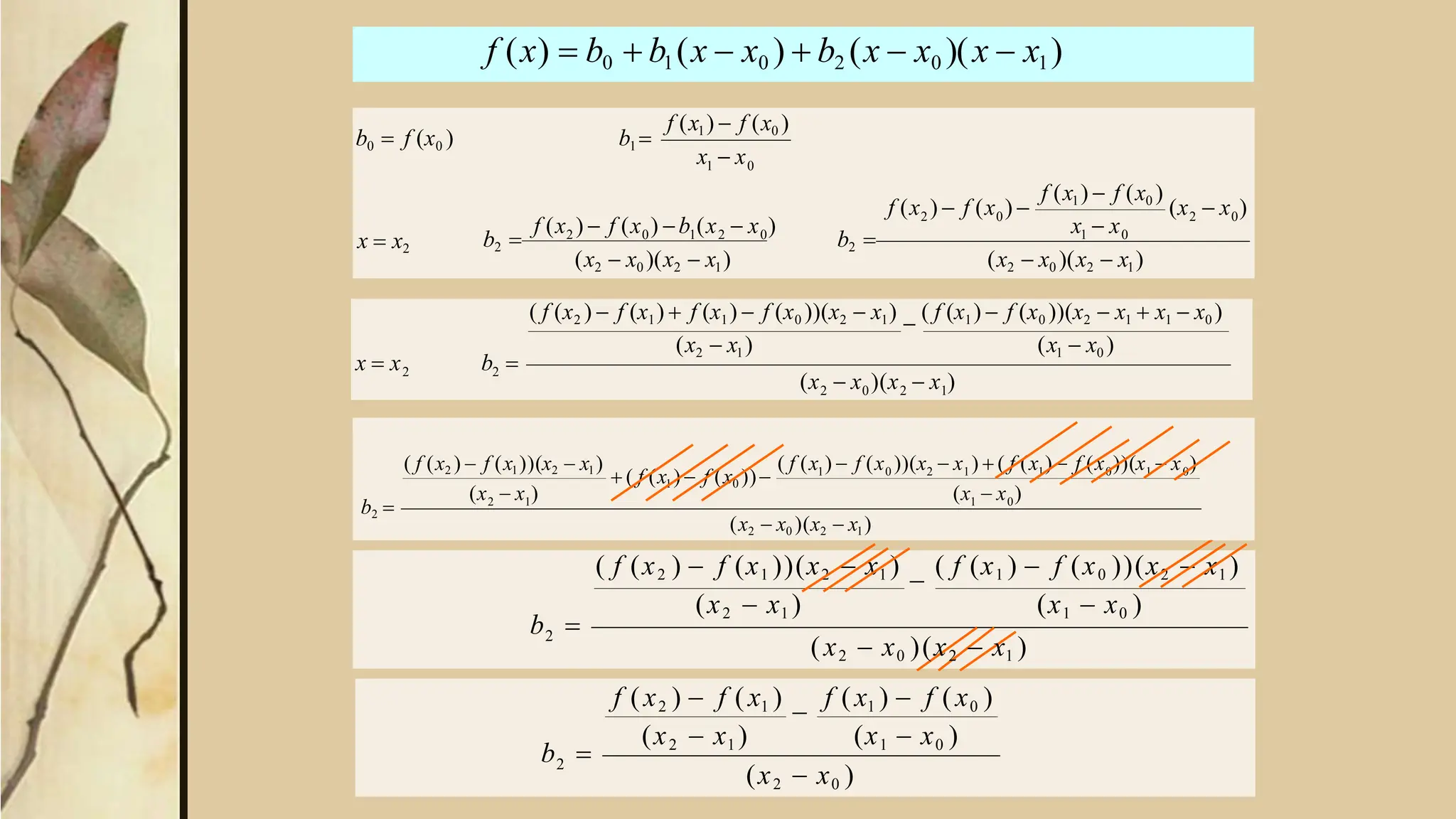
fn (x)  b0 b1(x  x0 ) b2(x  x0 )(x  x1)  bn (x  x0 )(x  x1) (x  xn1)
b0  f (x0 ) b1  f [x1, x0 ] b2  f [x2, x1, x0 ] … bn  f [xn , xn1, ,x1,x0 ]
i k
x  x
f [xi , xj ] f [xj , xk ]
f [xi , xj , xk ] 
0
1
n 0
x  x
n1 n2
n n1
n n1
f [x , x
f [x , x
, x ,…, x ]
,…, x ] f [x
,…, x1, x0 ] 
⁝

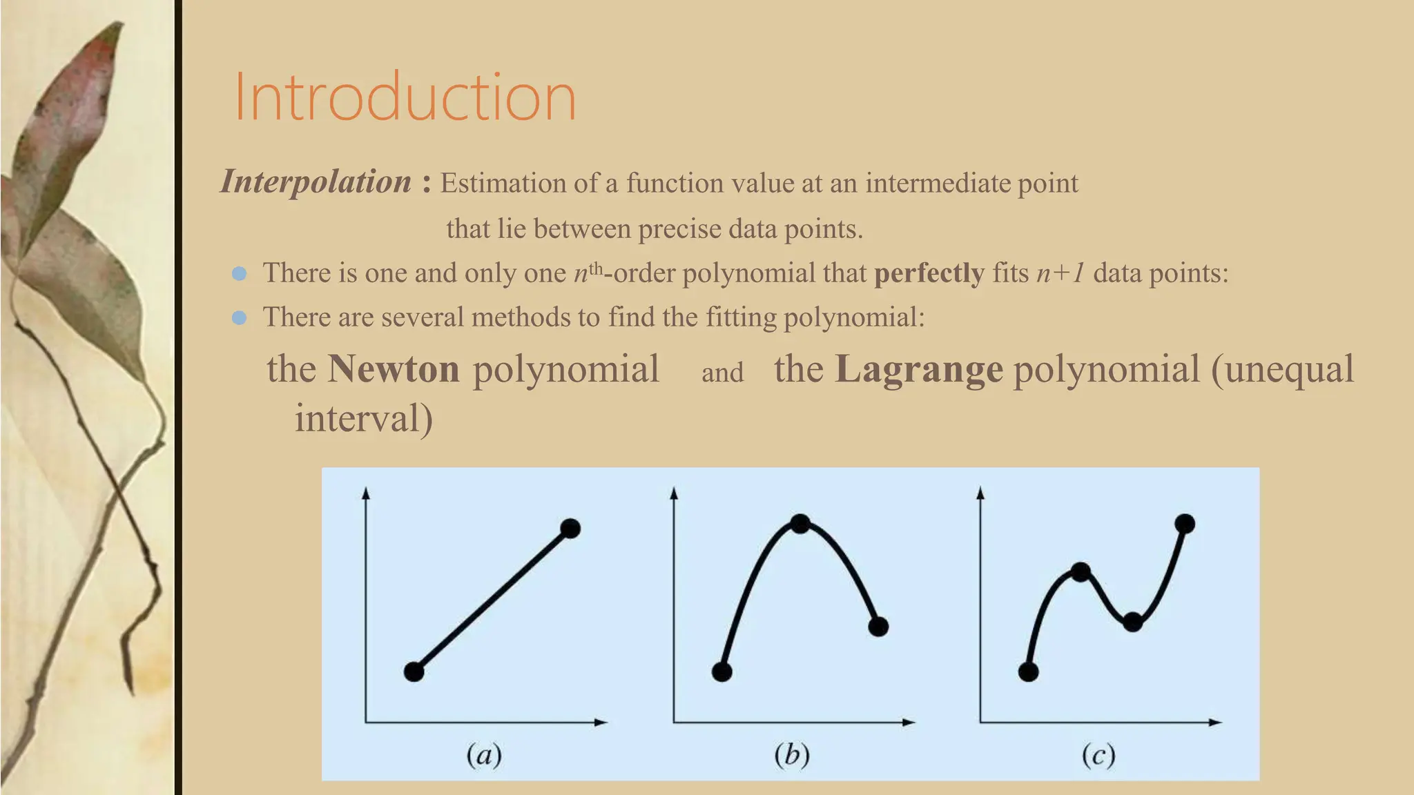
8. f1(x) = 2 + 6*(x-0) (based on x0 and x1)
f2(x) = 2 + 6*(x-0)+18(x-0)(x-2) (based on x0, x1 and x2)
f3(x) = 2 + 6*(x-0)+18(x-0)(x-2)+9(x-0)(x-2)(x-3) (based on x0, x1, x2, and x3)
f4(x) = 2 + 6x +18x(x-2) +9x(x-2)(x-3) +1x(x-2)(x-3)(x-4) (based on x0, x1, x2, x3, and x4)
= x4 – x2 + 2
EXAMPLE
DIVIDED DIFFERENCE TABLE
xi f(xi) f[xi,xj] f[xi,xj,xk] f[x,x,x,x] f[x...x]
x0=0 2
x1=2 14 6
x2=3 74 60 18
x3=4 242 168 54 9
x4=5 602 360 96 14 1
xi f(xi) f[xi,xj] f[xi,xj,xk] f[x,x,x,x]
x0 f(x0)
x1 f(x1) f[x1,x0]
x2 f(x2) f[x2,x1] f[x2,x1,x0]
x3 f(x3) f[x3,x2] f[x3,x2,x1] f[x3,x2,x1,x0]
x4 f(x4) f[x4,x3] f[x4,x3,x2] f[x4,x3,x2,x1]

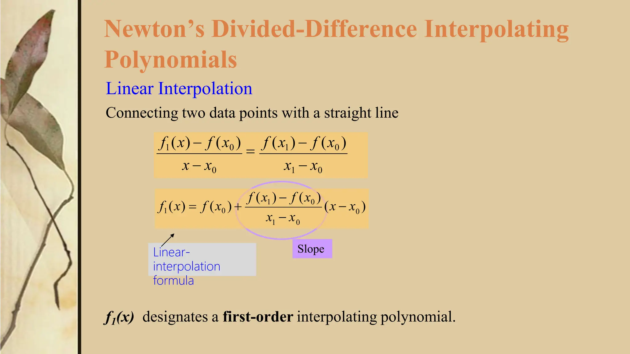
9. Given:
x0=1 f(x0)=ln(1) = 0
x1=e f(x1)=ln(2.72) = 1
x2=e2 f(x2)=ln(7.39) = 2
Estimate ln(2) = ?
using interpolation
Find f(x) first
xi f(xi)
x0=1 0
x1=2.72 1
x2=7.39 2
f[xi,xj] f[xi,xj xk]
.58
.214 -.057
f(x) = 0.58(x-1)
-0.057(x-1)(x-
2.72)
Then calculate
f(2)=0.58(2-1)-0.057(2-1)(2-
2.72)
= 0.621
[ TRUE ln(2) = 0.6931 ]
Example

10. Lagrange Interpolating Polynomials
• The Lagrange interpolating polynomial is simply a reformulation of the Newton’s polynomial that avoids the
computation of divided differences:
• Above formula can be easily verified by plugging in x0, x1…in the equation one at a time and checking if the
equality is satisfied.
n
j
i
n
xi  xj
x  x

j0
ji
L (x) 
fn (x)  Li (x) f (xi )
i0
1
1 0
0
0
1
1 f (x )
f (x ) 
x0  x1 x  x
x  x x  x
f (x) 
0 1
1
2
1 0 1
2
0
0
2
0 1 0
1 2
2
f (x2 )
f (x )
f (x )
x2  x0 x2 x1
x  x x  x 


x  x x x 
x  x x  x 

x  x x x 
x  x x  x 
f (x) 

11. Avisual depiction of the rationale behind
the Lagrange polynomial . The figure
shows a second order case:
Each of the three terms passes through
one of the data points and zero at the
other two. The summation of the three
terms must, therefore, be unique second
order polynomial f2(x) that passes exactly
through three points.
0 1
1
2
1 0 1
0 2
1 2
f (x2 )
f (x )
f (x0 )
x2  x0 x2 x1 
x  x x  x 


x  x x x 
x  x x  x 

x0  x1 x0 x2 
x  x x  x 
f2 (x) 


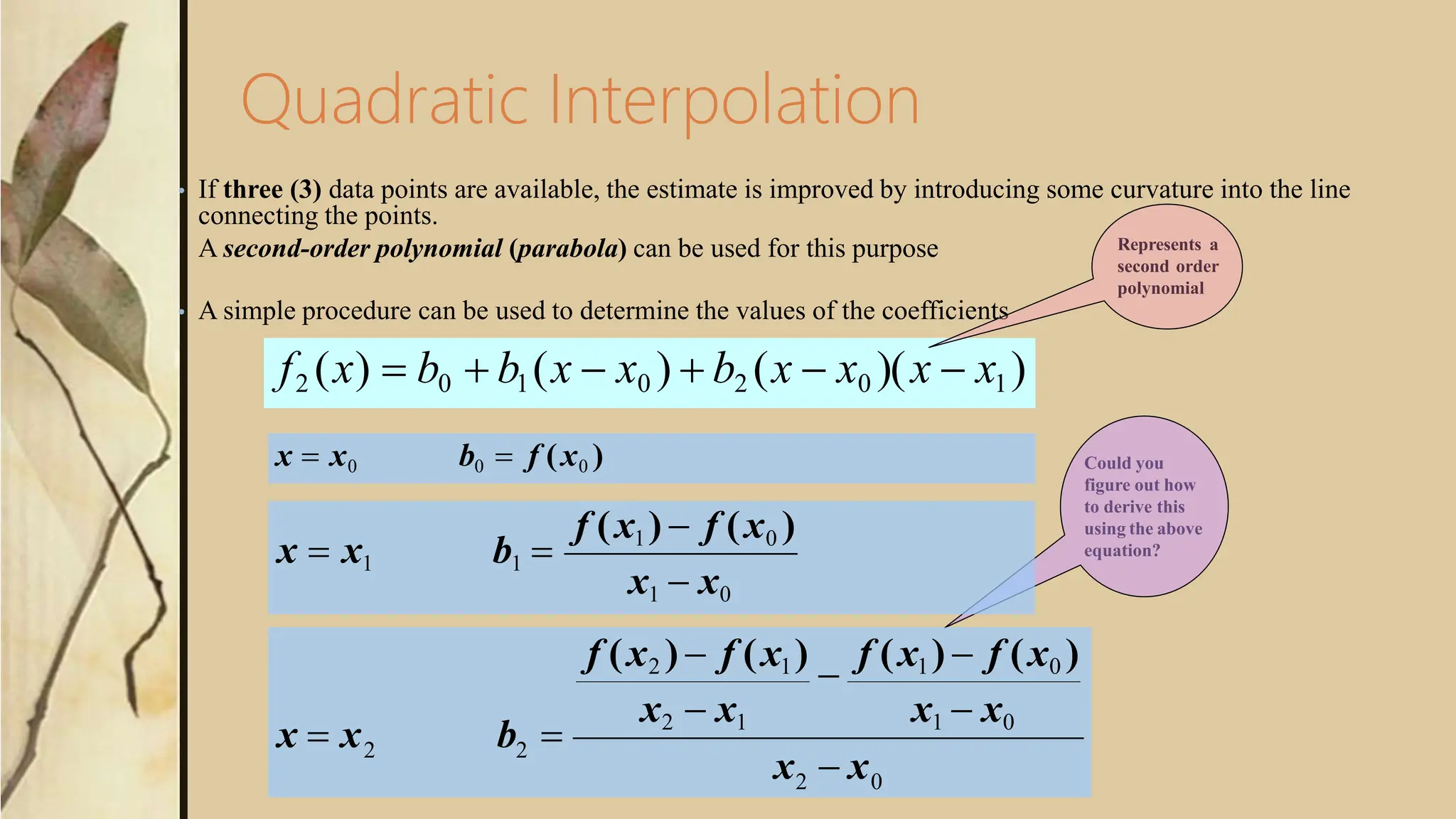
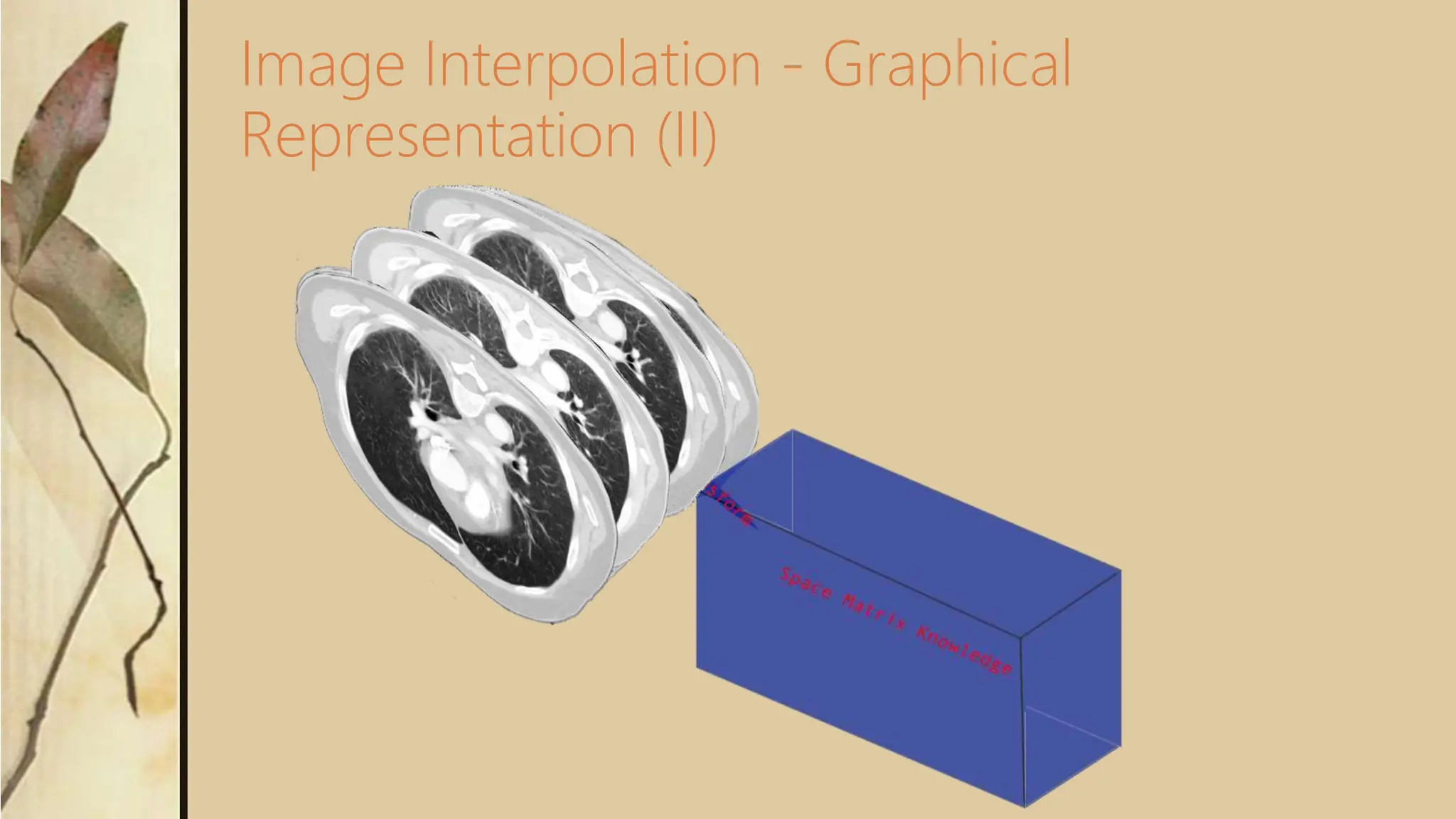
12. Image Interpolation - Theory
⚫ [IDEA]
⚫ In order to provide a richer environment we are thinking of using
interpolation methods that will generate “artificial images” thus revealing
hidden information.
⚫ [RADON RECONSTRUCTION]
⚫ Radon reconstruction is the technique in which the object is reconstructed
from its projections. This reconstruction method is based on approximating
the inverse Radon Transform.
⚫ [RADON Transform]
⚫ The 2-D Radon transform is the mathematical relationship which maps the
spatial domain (x,y) to the Radon domain (p,phi). The Radon transform
consists of taking a line integral along a line (ray) which passes through the
object space. The radon transform is expressed mathematically as:

{R
}( p,
)  
(x, y)(xcos ysin p)dxdy


13. Image Interpolation - Graphical
Representation (I)
y0 d
0  0
Rz (x,90)  
(x, y, z )dy
y0
l
0  0
Rz (y,0)  
(x, y, z )dx
0

14. Image Interpolation - Graphical
Representation (II)

15. Thank Y
ou