Download as PDF, PPTX


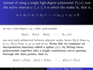
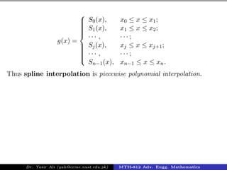
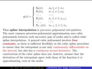
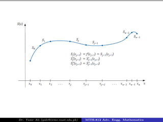


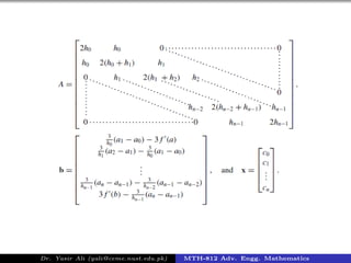

The document discusses cubic spline interpolation, a method used in engineering mathematics to estimate values at intermediate points based on provided data points. It highlights the advantages of using multiple low-degree polynomials over a single high-degree polynomial to avoid numerical instability, particularly when dealing with a large number of data points. Cubic spline interpolation ensures continuity and differentiability while fitting polynomials between each pair of nodes.