Part 5b:
INTERPOLATION
–
–
–
–

Newton’s Divided-Differences
Lagrange Polynomial Interpolation
Inverse Interpolation
Spline Interpolation
Introduction:
 Interpolation is the process of estimating intermediate values
between precisely defined data points.
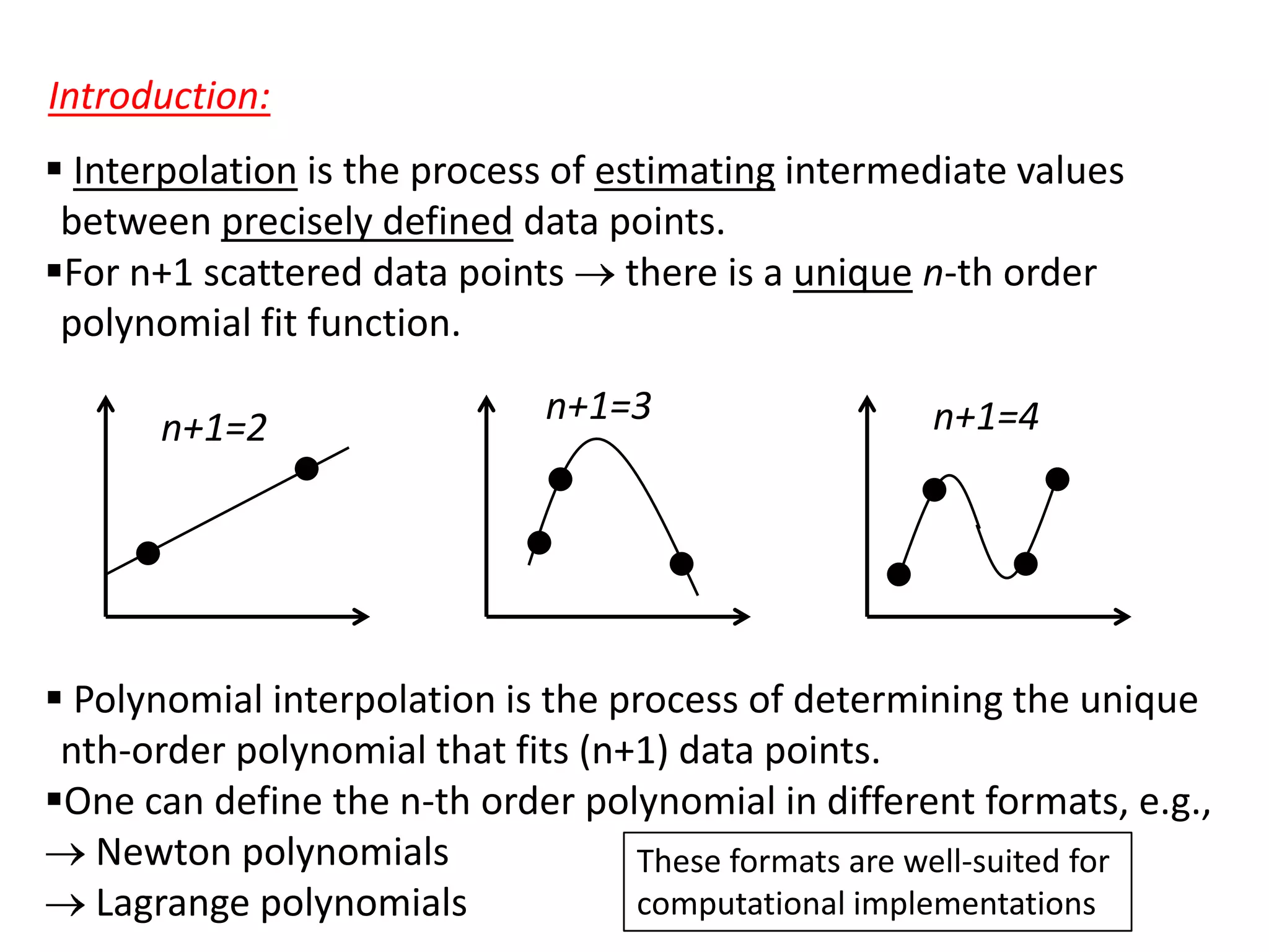
For n+1 scattered data points there is a unique n-th order
polynomial fit function.

n+1=2

n+1=3

n+1=4

 Polynomial interpolation is the process of determining the unique
nth-order polynomial that fits (n+1) data points.
One can define the n-th order polynomial in different formats, e.g.,
Newton polynomials
These formats are well-suited for
computational implementations
Lagrange polynomials
Newton’s Divided Differences
 One of the most popular interpolating functions
Linear interpolation:
 Simplest form of interpolation: connect two data points by a
underlying
straight line, and estimate the intermediate value.
f(x)

f1(x) fit function

Similarity of the triangles:
f1 ( x) f ( x0 )
x x0

f(x1)
f1(x)
f(x0)

f ( x1 ) f ( x0 )
x1 x0
finite divided difference
of first derivative

x0

x

x1

f1 ( x)

f ( x0 )

f ( x1 ) f ( x0 )
( x x0 )
x1 x0

for data points

f1 ( xi )

function

f ( xi )

represents the first
order interpolation

linear interpolation formula
Quadratic interpolation:
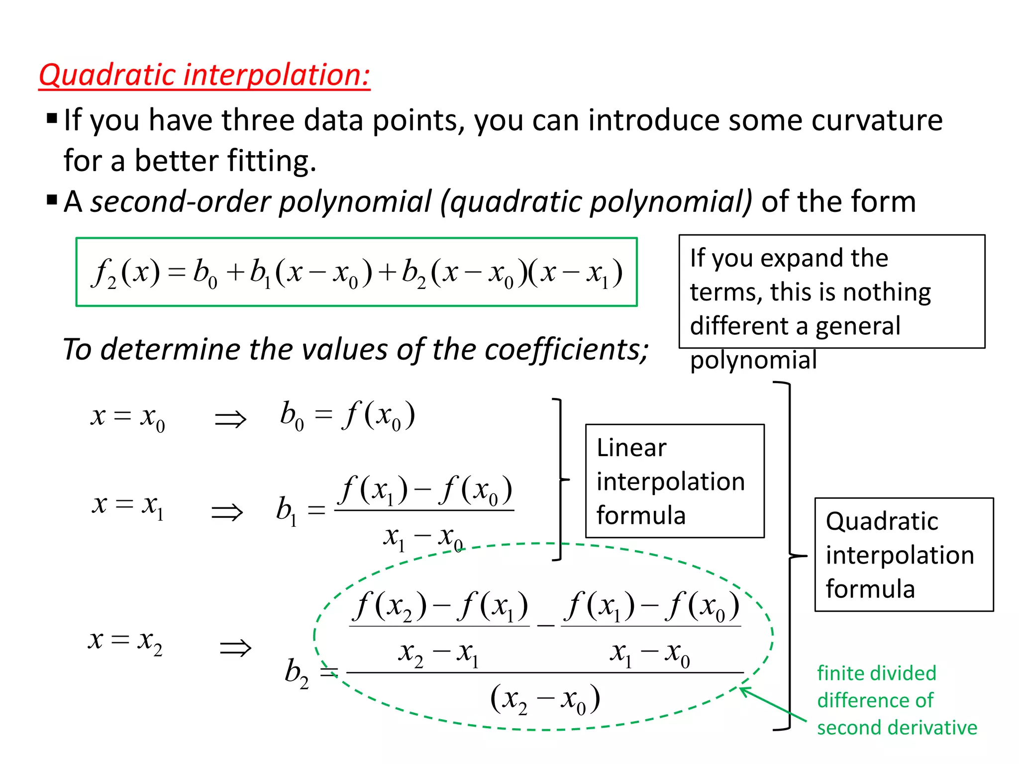
 If you have three data points, you can introduce some curvature
for a better fitting.
 A second-order polynomial (quadratic polynomial) of the form
f 2 ( x) b0 b1 ( x x0 ) b2 ( x x0 )( x x1 )

To determine the values of the coefficients;
x

x

x

x0

x1

x2

b0

f ( x0 )

b1

f ( x1 ) f ( x0 )
x1 x0

b2

If you expand the
terms, this is nothing
different a general
polynomial

Linear
interpolation
formula

f ( x2 ) f ( x1 ) f ( x1 ) f ( x0 )
x2 x1
x1 x0
( x2 x0 )

Quadratic
interpolation
formula
finite divided
difference of
second derivative
General form of Newton’s interpolating polynomials:
In general, to fit an n-the order Newton’s polynomial to (n+1) data
points:
f n ( x) b0 b1 ( x x0 ) b2 ( x x0 )( x x1 ) .. bn ( x x0 )( x x1 )..( x xn 1 )

where the coefficients:
b0

f [ x0 ]

b1

f [ x1 , x0 ]

b2

f [ x2 , x1 , x0 ]

data points

n-th finite divided difference:

…
bn

brackets represent the
function evaluations for
finite divided-differences

f [ xn , xn 1 ,.., x1 , x0 ]

f [ xn , xn 1 ,.., x1 , x0 ]
f [ xn , xn 1 ,.., x1 ] f [ xn 1 ,.., x1 , x0 ]
( xn x0 )
 These differences can be evaluated for the coefficients and
substituted into the fitting function.
f n ( x)

f ( x0 ) ( x x0 ) f [ x1 , x0 ] ( x x0 )(x x1 ) f [ x2 , x1 , x0 ]

.. ( x x0 )(x x1 )..(x xn 1 ) f [ xn , xn 1 ,.., x0 ]

 x values are not need to be equally
spaced.
 x values are not necessarily in order.

Newton’s divideddifference interpolating
polynomial
Error for Newton’s interpolating polynomials:
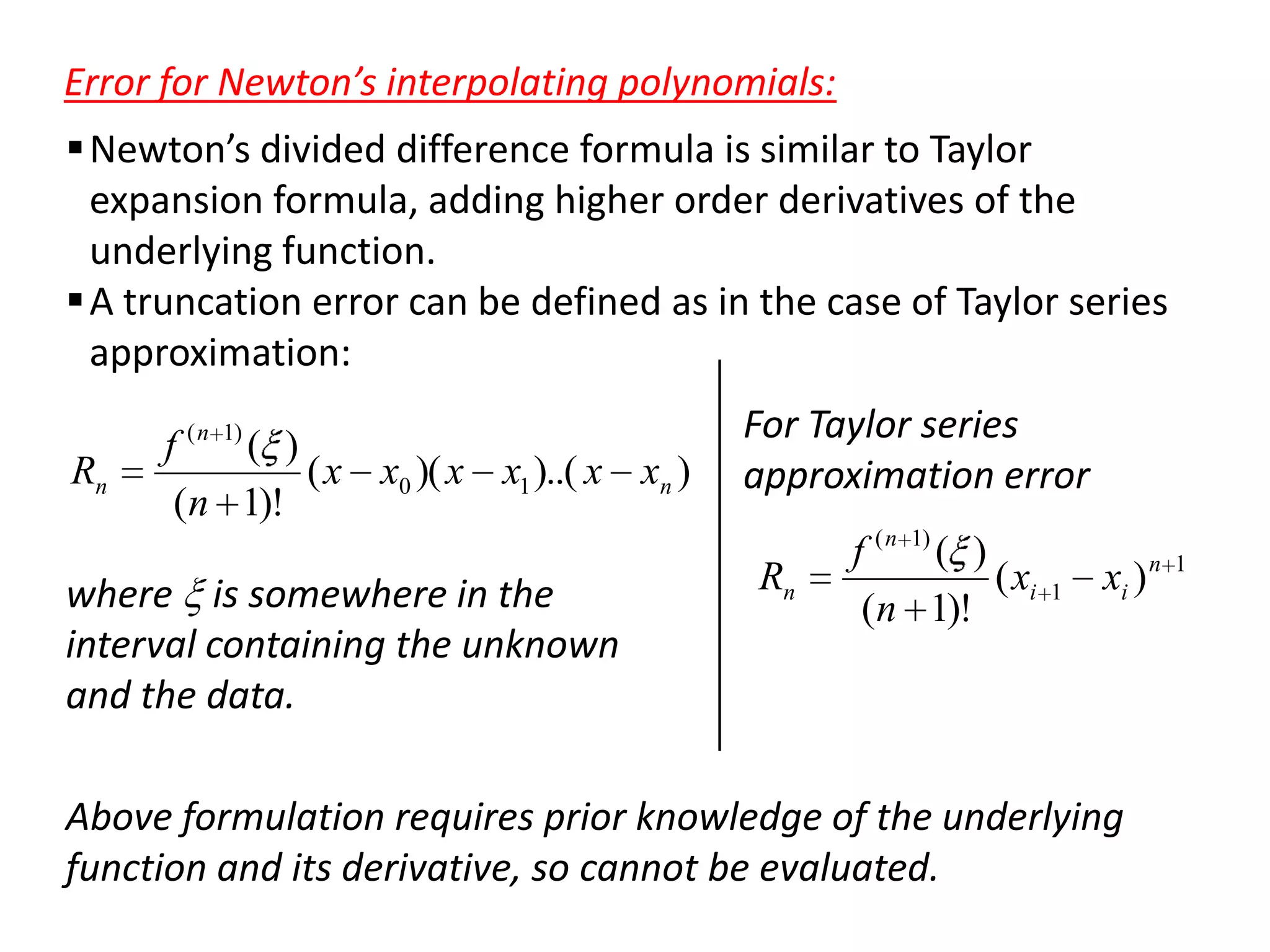
 Newton’s divided difference formula is similar to Taylor
expansion formula, adding higher order derivatives of the
underlying function.
 A truncation error can be defined as in the case of Taylor series
approximation:
Rn

f ( n 1) ( )
( x x0 )( x x1 )..( x xn )
(n 1)!

where is somewhere in the
interval containing the unknown
and the data.

For Taylor series
approximation error
Rn

f ( n 1) ( )
( xi
(n 1)!

1

xi ) n

Above formulation requires prior knowledge of the underlying
function and its derivative, so cannot be evaluated.

1
An alternative formulation that does not require prior knowledge
of the underlying function:
Rn

f [ x, xn , xn 1 ,..., x0 ]( x x0 )( x x1 )..( x xn )
(n+1)th finite
divided difference

 One more data point (xn+1) is needed to evaluate the equation.
Rn

f [ xn 1 , xn , xn 1 ,..., x0 ]( x x0 )( x x1 )..( x xn )

This relationship is equivalent to
Rn

f n 1 ( x)

f n 1 ( x)

f n ( x)

f n ( x) Rn

(next estimate) - (current estimate)

increment added to the (n)th order case
to calculate (n+1)th order case is equal to
the error for the n-th order case.
Lagrange Polynomial Interpolation
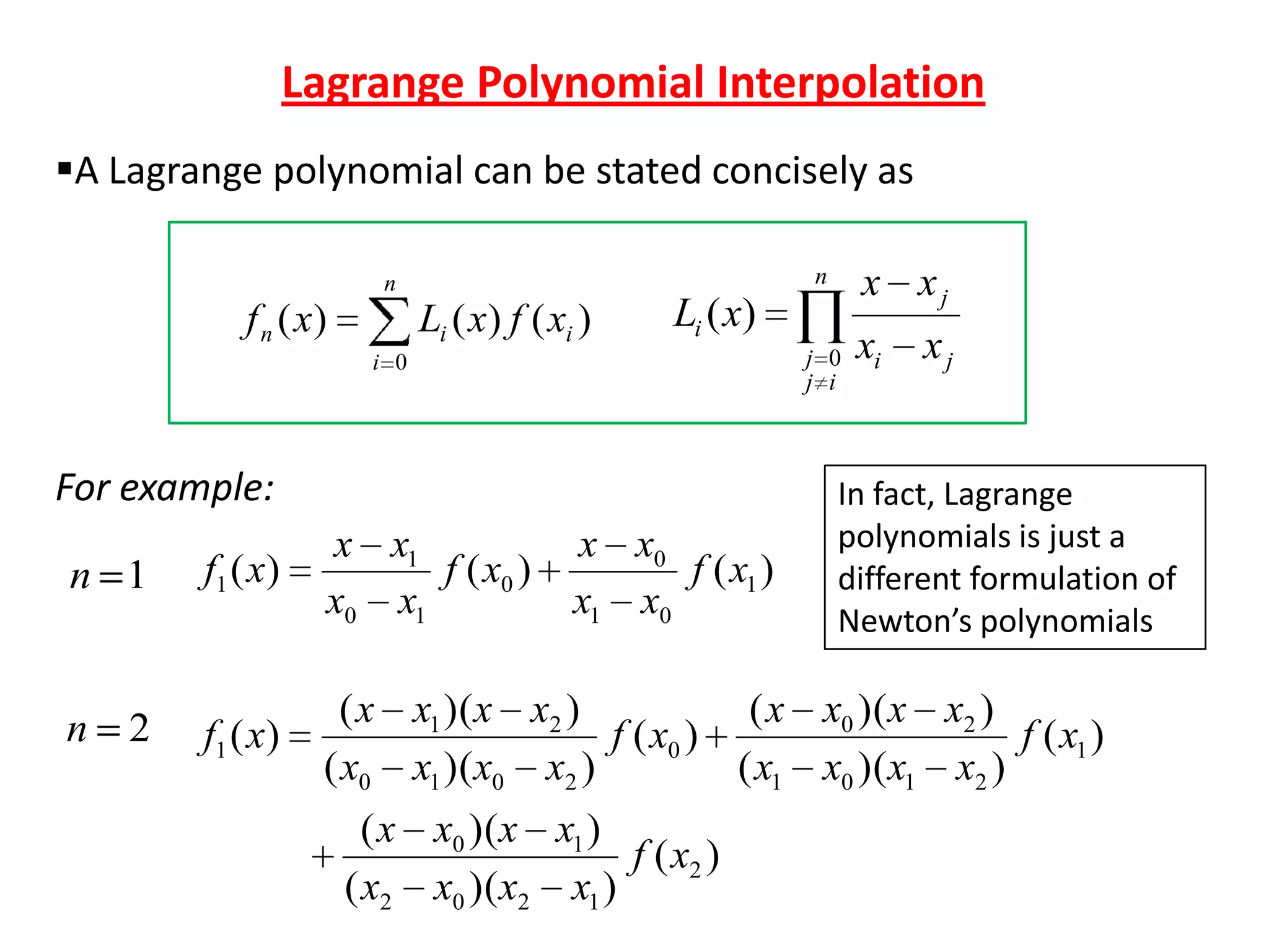
A Lagrange polynomial can be stated concisely as

f n ( x)

Li ( x) f ( xi )

Li ( x)
j 0
j i

i 0

For example:
n 1

n

2

x xj

n

n

x x0
f ( x1 )
x1 x0

xi

xj

In fact, Lagrange
polynomials is just a
different formulation of
Newton’s polynomials

f1 ( x)

x x1
f ( x0 )
x0 x1

f1 ( x)

( x x0 )(x x2 )
( x x1 )(x x2 )
f ( x0 )
f ( x1 )
( x0 x1 )(x0 x2 )
( x1 x0 )(x1 x2 )
( x x0 )(x x1 )
f ( x2 )
( x2 x0 )(x2 x1 )
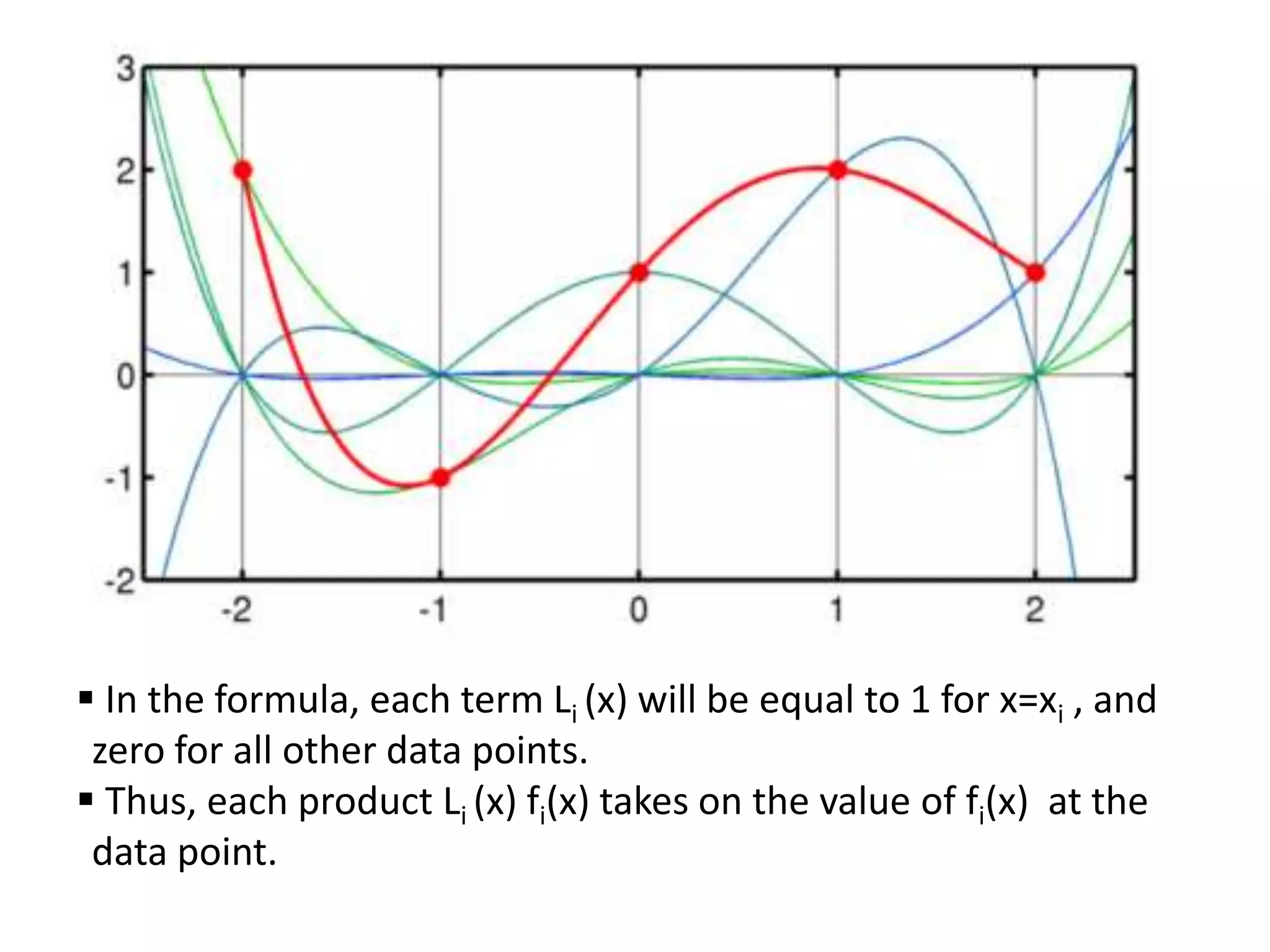
 In the formula, each term Li (x) will be equal to 1 for x=xi , and
zero for all other data points.
 Thus, each product Li (x) fi(x) takes on the value of fi(x) at the
data point.
Error is defined same as before
Rn

f [ x, xn , xn 1 ,..., x0 ]( x x0 )( x x1 )..( x xn )

(An additional point (xn+1) is needed for evaluation)

In summary:
Newton’s method is preferable for exploratory computations (n
is not known a priori).
> Newton method has advantages because of the insight for the
behavior between different orders (consider Taylor series).
> Error estimate in Newton method can easily be implemented
as it employs a finite difference.
Lagrange method is preferable when only one interpolation is
performed (order n is known a priori),
> It is easier for computational implementation.
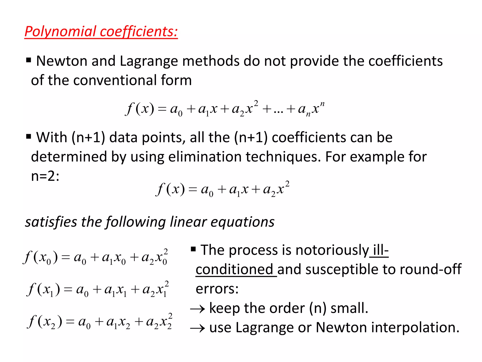
Polynomial coefficients:
 Newton and Lagrange methods do not provide the coefficients
of the conventional form
f ( x)

a0

a1 x a2 x 2 ... an x n

 With (n+1) data points, all the (n+1) coefficients can be
determined by using elimination techniques. For example for
n=2:
2
f ( x)

a0

a1 x a2 x

satisfies the following linear equations
f ( x0 )

a0

a1 x0

2
a2 x0

f ( x1 )

a0

a1 x1

a2 x12

f ( x2 )

a0

a1 x2

2
a 2 x2

 The process is notoriously illconditioned and susceptible to round-off
errors:
keep the order (n) small.
use Lagrange or Newton interpolation.
Inverse Interpolation
dependant variable
independent variable
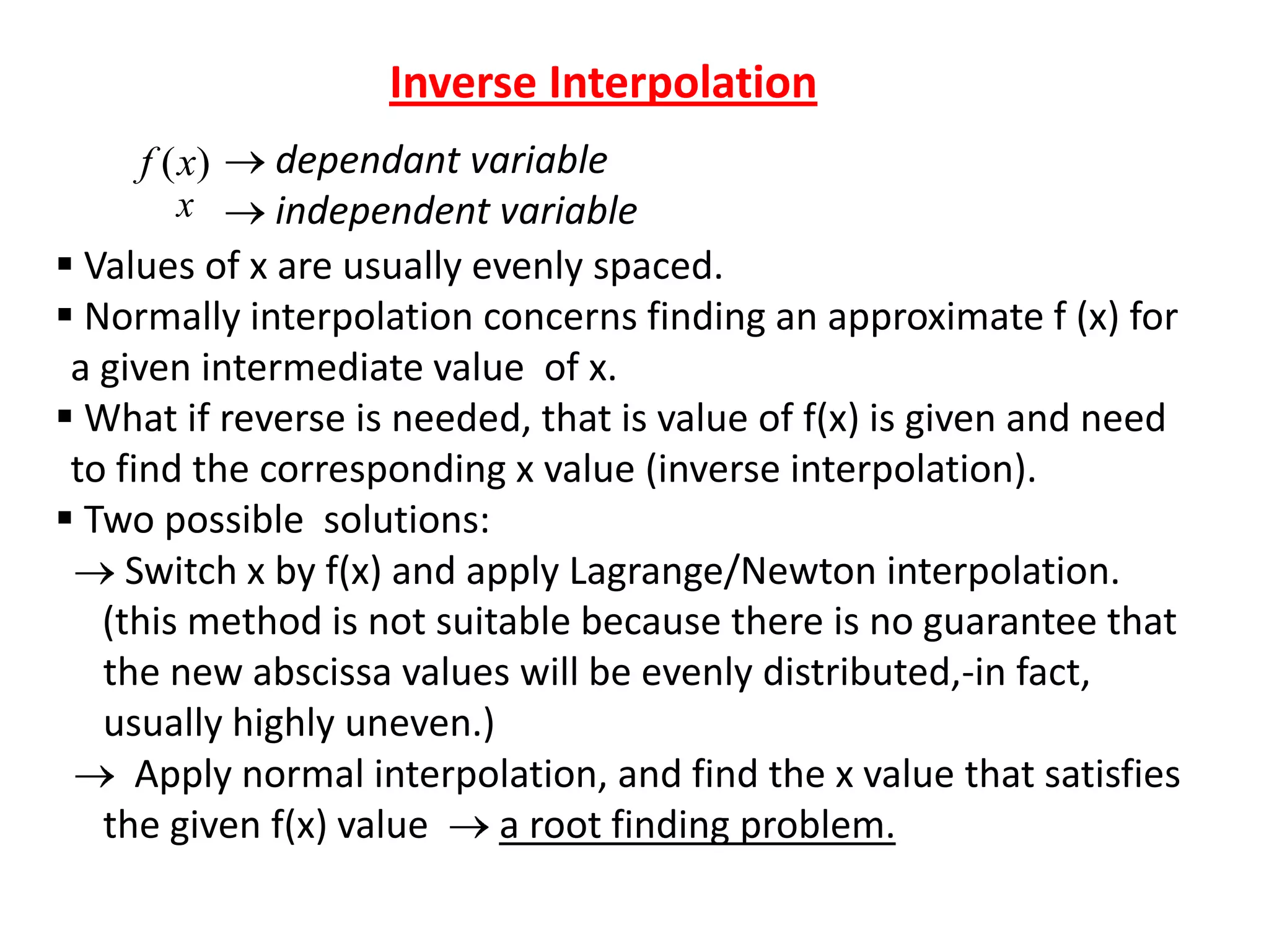
 Values of x are usually evenly spaced.
 Normally interpolation concerns finding an approximate f (x) for
a given intermediate value of x.
 What if reverse is needed, that is value of f(x) is given and need
to find the corresponding x value (inverse interpolation).
 Two possible solutions:
Switch x by f(x) and apply Lagrange/Newton interpolation.
(this method is not suitable because there is no guarantee that
the new abscissa values will be evenly distributed,-in fact,
usually highly uneven.)
Apply normal interpolation, and find the x value that satisfies
the given f(x) value
a root finding problem.
f (x)
x
Equally spaced data:
 Newton/Lagrange methods are compatible for arbitrarily spaced
data
 Before the computer era, equally spaced data had to be
used, but computer implementation of these methods do not
require it anymore.
 Evenly spaced data is required for other applications
too, e.g., numerical differentiation and integration.
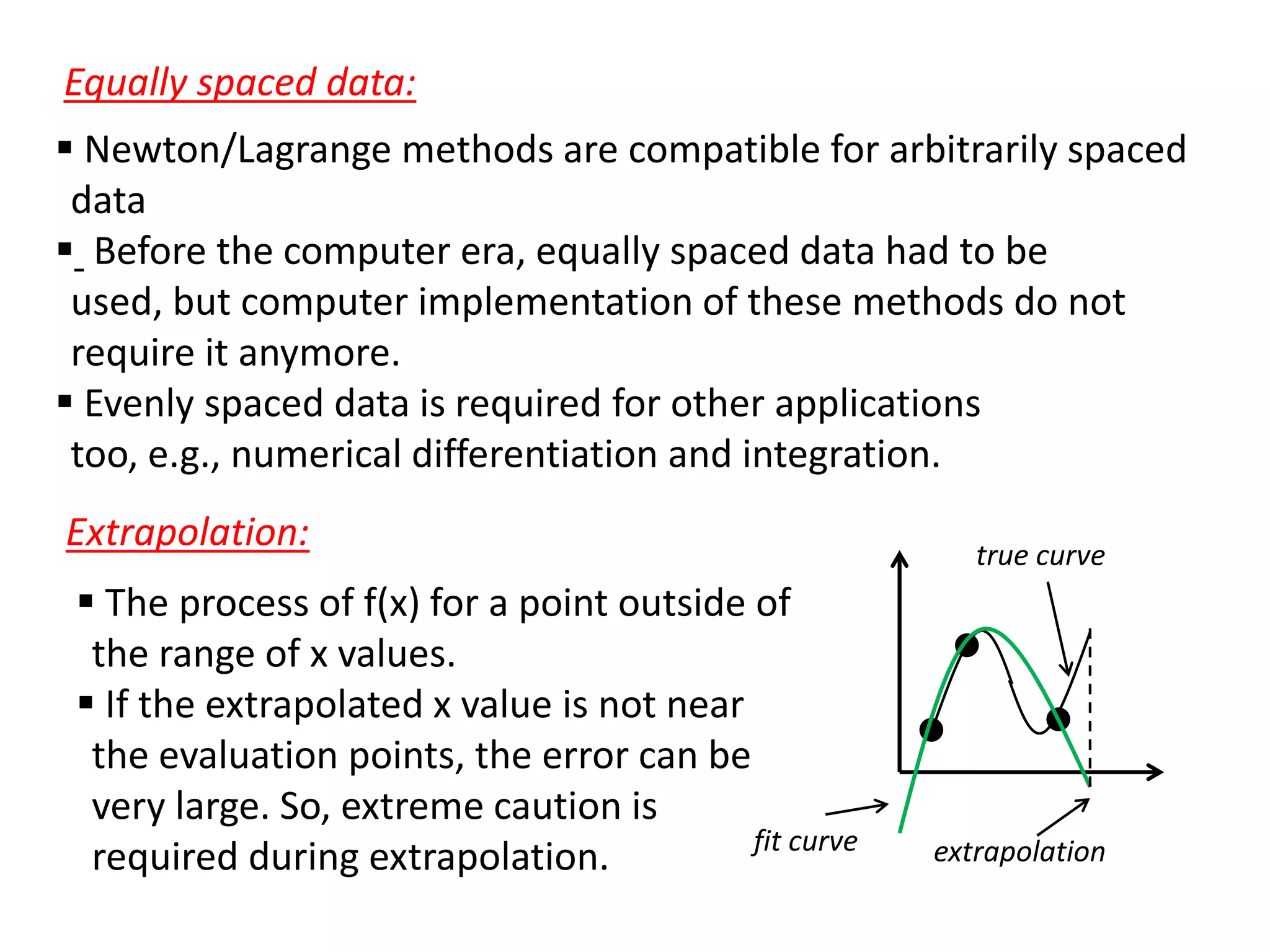
Extrapolation:
 The process of f(x) for a point outside of
the range of x values.
 If the extrapolated x value is not near
the evaluation points, the error can be
very large. So, extreme caution is
fit curve
required during extrapolation.

true curve

extrapolation
Spline Interpolation
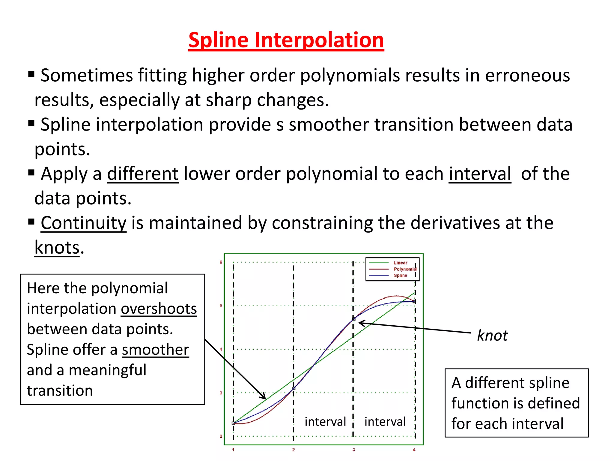
 Sometimes fitting higher order polynomials results in erroneous
results, especially at sharp changes.
 Spline interpolation provide s smoother transition between data
points.
 Apply a different lower order polynomial to each interval of the
data points.
 Continuity is maintained by constraining the derivatives at the
knots.
Here the polynomial
interpolation overshoots
between data points.
Spline offer a smoother
and a meaningful
transition

knot

interval

interval

A different spline
function is defined
for each interval
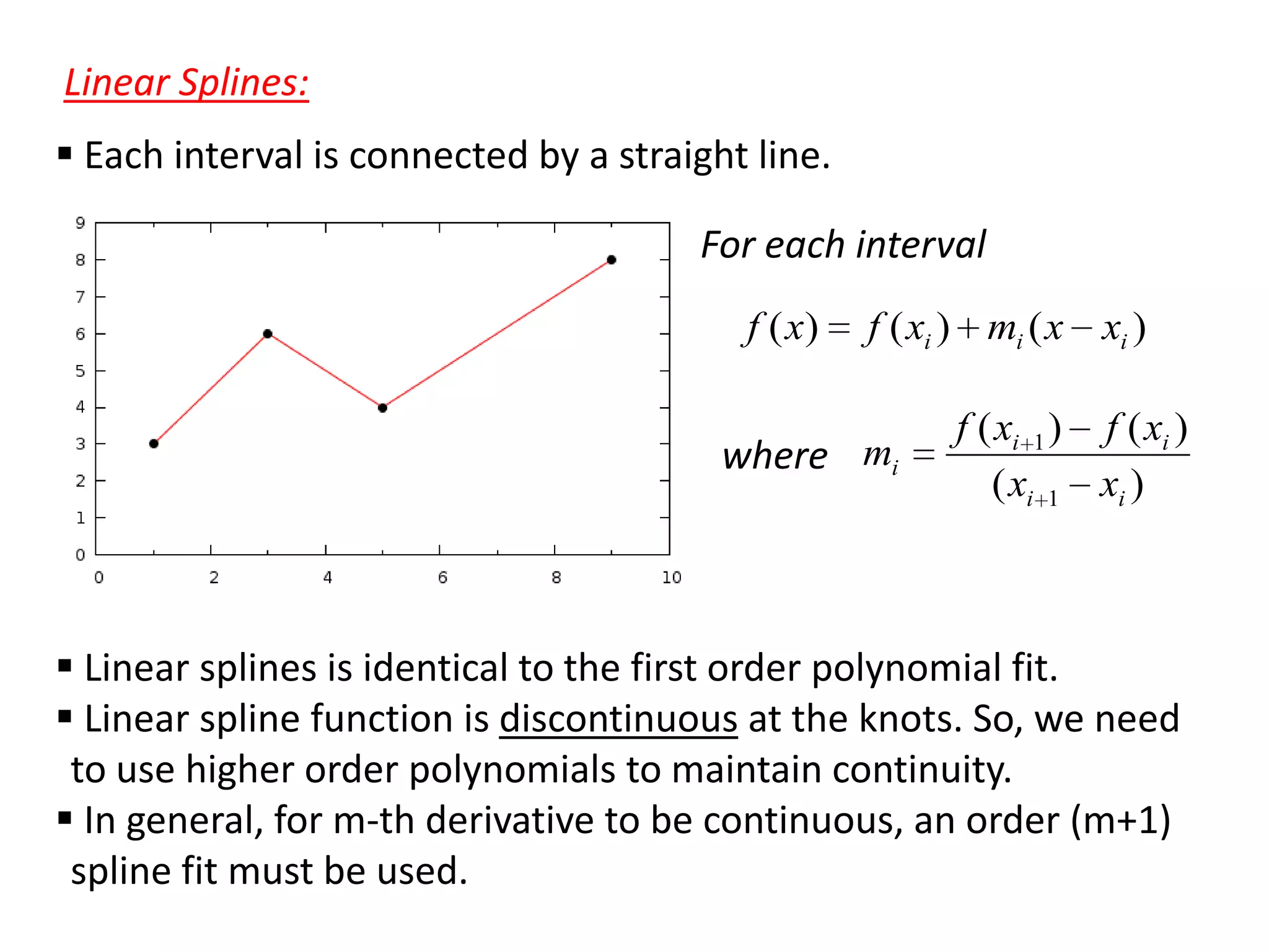
Linear Splines:
 Each interval is connected by a straight line.
For each interval
f ( x)

f ( xi ) mi ( x xi )

where mi

f ( xi 1 ) f ( xi )
( xi 1 xi )

 Linear splines is identical to the first order polynomial fit.
 Linear spline function is discontinuous at the knots. So, we need
to use higher order polynomials to maintain continuity.
 In general, for m-th derivative to be continuous, an order (m+1)
spline fit must be used.
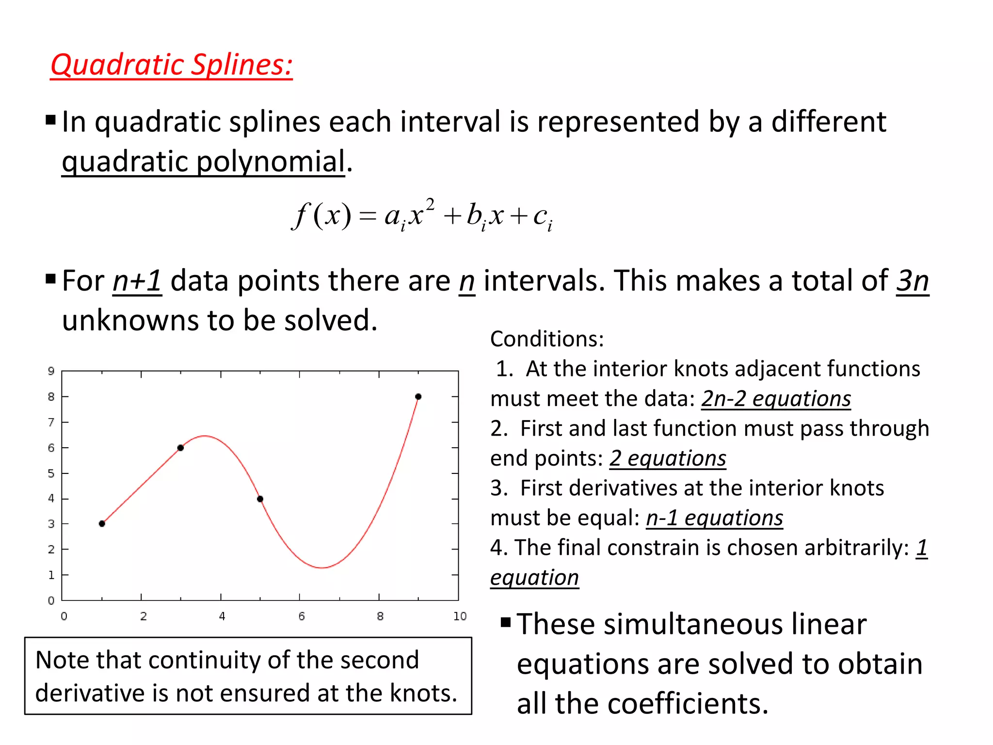
Quadratic Splines:
In quadratic splines each interval is represented by a different
quadratic polynomial.
f ( x)

ai x 2

bi x ci

For n+1 data points there are n intervals. This makes a total of 3n
unknowns to be solved.
Conditions:
1. At the interior knots adjacent functions
must meet the data: 2n-2 equations
2. First and last function must pass through
end points: 2 equations
3. First derivatives at the interior knots
must be equal: n-1 equations
4. The final constrain is chosen arbitrarily: 1
equation

Note that continuity of the second
derivative is not ensured at the knots.

These simultaneous linear
equations are solved to obtain
all the coefficients.
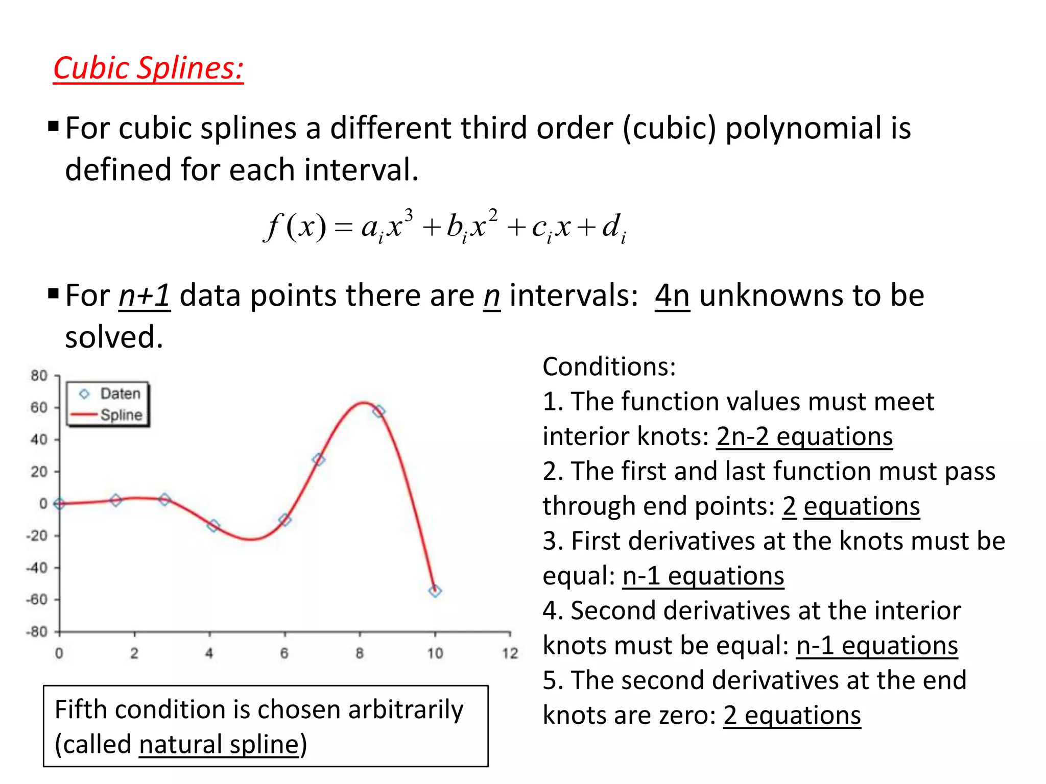
Cubic Splines:
For cubic splines a different third order (cubic) polynomial is
defined for each interval.
f ( x)

ai x 3 bi x 2

ci x d i

For n+1 data points there are n intervals: 4n unknowns to be
solved.

Fifth condition is chosen arbitrarily
(called natural spline)

Conditions:
1. The function values must meet
interior knots: 2n-2 equations
2. The first and last function must pass
through end points: 2 equations
3. First derivatives at the knots must be
equal: n-1 equations
4. Second derivatives at the interior
knots must be equal: n-1 equations
5. The second derivatives at the end
knots are zero: 2 equations

Es272 ch5b

  • 1.
    Part 5b: INTERPOLATION – – – – Newton’s Divided-Differences LagrangePolynomial Interpolation Inverse Interpolation Spline Interpolation
  • 2.
    Introduction:  Interpolation isthe process of estimating intermediate values between precisely defined data points. For n+1 scattered data points there is a unique n-th order polynomial fit function. n+1=2 n+1=3 n+1=4  Polynomial interpolation is the process of determining the unique nth-order polynomial that fits (n+1) data points. One can define the n-th order polynomial in different formats, e.g., Newton polynomials These formats are well-suited for computational implementations Lagrange polynomials
  • 3.
    Newton’s Divided Differences One of the most popular interpolating functions Linear interpolation:  Simplest form of interpolation: connect two data points by a underlying straight line, and estimate the intermediate value. f(x) f1(x) fit function Similarity of the triangles: f1 ( x) f ( x0 ) x x0 f(x1) f1(x) f(x0) f ( x1 ) f ( x0 ) x1 x0 finite divided difference of first derivative x0 x x1 f1 ( x) f ( x0 ) f ( x1 ) f ( x0 ) ( x x0 ) x1 x0 for data points f1 ( xi ) function f ( xi ) represents the first order interpolation linear interpolation formula
  • 4.
    Quadratic interpolation:  Ifyou have three data points, you can introduce some curvature for a better fitting.  A second-order polynomial (quadratic polynomial) of the form f 2 ( x) b0 b1 ( x x0 ) b2 ( x x0 )( x x1 ) To determine the values of the coefficients; x x x x0 x1 x2 b0 f ( x0 ) b1 f ( x1 ) f ( x0 ) x1 x0 b2 If you expand the terms, this is nothing different a general polynomial Linear interpolation formula f ( x2 ) f ( x1 ) f ( x1 ) f ( x0 ) x2 x1 x1 x0 ( x2 x0 ) Quadratic interpolation formula finite divided difference of second derivative
  • 5.
    General form ofNewton’s interpolating polynomials: In general, to fit an n-the order Newton’s polynomial to (n+1) data points: f n ( x) b0 b1 ( x x0 ) b2 ( x x0 )( x x1 ) .. bn ( x x0 )( x x1 )..( x xn 1 ) where the coefficients: b0 f [ x0 ] b1 f [ x1 , x0 ] b2 f [ x2 , x1 , x0 ] data points n-th finite divided difference: … bn brackets represent the function evaluations for finite divided-differences f [ xn , xn 1 ,.., x1 , x0 ] f [ xn , xn 1 ,.., x1 , x0 ] f [ xn , xn 1 ,.., x1 ] f [ xn 1 ,.., x1 , x0 ] ( xn x0 )
  • 6.
     These differencescan be evaluated for the coefficients and substituted into the fitting function. f n ( x) f ( x0 ) ( x x0 ) f [ x1 , x0 ] ( x x0 )(x x1 ) f [ x2 , x1 , x0 ] .. ( x x0 )(x x1 )..(x xn 1 ) f [ xn , xn 1 ,.., x0 ]  x values are not need to be equally spaced.  x values are not necessarily in order. Newton’s divideddifference interpolating polynomial
  • 7.
    Error for Newton’sinterpolating polynomials:  Newton’s divided difference formula is similar to Taylor expansion formula, adding higher order derivatives of the underlying function.  A truncation error can be defined as in the case of Taylor series approximation: Rn f ( n 1) ( ) ( x x0 )( x x1 )..( x xn ) (n 1)! where is somewhere in the interval containing the unknown and the data. For Taylor series approximation error Rn f ( n 1) ( ) ( xi (n 1)! 1 xi ) n Above formulation requires prior knowledge of the underlying function and its derivative, so cannot be evaluated. 1
  • 8.
    An alternative formulationthat does not require prior knowledge of the underlying function: Rn f [ x, xn , xn 1 ,..., x0 ]( x x0 )( x x1 )..( x xn ) (n+1)th finite divided difference  One more data point (xn+1) is needed to evaluate the equation. Rn f [ xn 1 , xn , xn 1 ,..., x0 ]( x x0 )( x x1 )..( x xn ) This relationship is equivalent to Rn f n 1 ( x) f n 1 ( x) f n ( x) f n ( x) Rn (next estimate) - (current estimate) increment added to the (n)th order case to calculate (n+1)th order case is equal to the error for the n-th order case.
  • 9.
    Lagrange Polynomial Interpolation ALagrange polynomial can be stated concisely as f n ( x) Li ( x) f ( xi ) Li ( x) j 0 j i i 0 For example: n 1 n 2 x xj n n x x0 f ( x1 ) x1 x0 xi xj In fact, Lagrange polynomials is just a different formulation of Newton’s polynomials f1 ( x) x x1 f ( x0 ) x0 x1 f1 ( x) ( x x0 )(x x2 ) ( x x1 )(x x2 ) f ( x0 ) f ( x1 ) ( x0 x1 )(x0 x2 ) ( x1 x0 )(x1 x2 ) ( x x0 )(x x1 ) f ( x2 ) ( x2 x0 )(x2 x1 )
  • 10.
     In theformula, each term Li (x) will be equal to 1 for x=xi , and zero for all other data points.  Thus, each product Li (x) fi(x) takes on the value of fi(x) at the data point.
  • 11.
    Error is definedsame as before Rn f [ x, xn , xn 1 ,..., x0 ]( x x0 )( x x1 )..( x xn ) (An additional point (xn+1) is needed for evaluation) In summary: Newton’s method is preferable for exploratory computations (n is not known a priori). > Newton method has advantages because of the insight for the behavior between different orders (consider Taylor series). > Error estimate in Newton method can easily be implemented as it employs a finite difference. Lagrange method is preferable when only one interpolation is performed (order n is known a priori), > It is easier for computational implementation.
  • 12.
    Polynomial coefficients:  Newtonand Lagrange methods do not provide the coefficients of the conventional form f ( x) a0 a1 x a2 x 2 ... an x n  With (n+1) data points, all the (n+1) coefficients can be determined by using elimination techniques. For example for n=2: 2 f ( x) a0 a1 x a2 x satisfies the following linear equations f ( x0 ) a0 a1 x0 2 a2 x0 f ( x1 ) a0 a1 x1 a2 x12 f ( x2 ) a0 a1 x2 2 a 2 x2  The process is notoriously illconditioned and susceptible to round-off errors: keep the order (n) small. use Lagrange or Newton interpolation.
  • 13.
    Inverse Interpolation dependant variable independentvariable  Values of x are usually evenly spaced.  Normally interpolation concerns finding an approximate f (x) for a given intermediate value of x.  What if reverse is needed, that is value of f(x) is given and need to find the corresponding x value (inverse interpolation).  Two possible solutions: Switch x by f(x) and apply Lagrange/Newton interpolation. (this method is not suitable because there is no guarantee that the new abscissa values will be evenly distributed,-in fact, usually highly uneven.) Apply normal interpolation, and find the x value that satisfies the given f(x) value a root finding problem. f (x) x
  • 14.
    Equally spaced data: Newton/Lagrange methods are compatible for arbitrarily spaced data  Before the computer era, equally spaced data had to be used, but computer implementation of these methods do not require it anymore.  Evenly spaced data is required for other applications too, e.g., numerical differentiation and integration. Extrapolation:  The process of f(x) for a point outside of the range of x values.  If the extrapolated x value is not near the evaluation points, the error can be very large. So, extreme caution is fit curve required during extrapolation. true curve extrapolation
  • 15.
    Spline Interpolation  Sometimesfitting higher order polynomials results in erroneous results, especially at sharp changes.  Spline interpolation provide s smoother transition between data points.  Apply a different lower order polynomial to each interval of the data points.  Continuity is maintained by constraining the derivatives at the knots. Here the polynomial interpolation overshoots between data points. Spline offer a smoother and a meaningful transition knot interval interval A different spline function is defined for each interval
  • 16.
    Linear Splines:  Eachinterval is connected by a straight line. For each interval f ( x) f ( xi ) mi ( x xi ) where mi f ( xi 1 ) f ( xi ) ( xi 1 xi )  Linear splines is identical to the first order polynomial fit.  Linear spline function is discontinuous at the knots. So, we need to use higher order polynomials to maintain continuity.  In general, for m-th derivative to be continuous, an order (m+1) spline fit must be used.
  • 17.
    Quadratic Splines: In quadraticsplines each interval is represented by a different quadratic polynomial. f ( x) ai x 2 bi x ci For n+1 data points there are n intervals. This makes a total of 3n unknowns to be solved. Conditions: 1. At the interior knots adjacent functions must meet the data: 2n-2 equations 2. First and last function must pass through end points: 2 equations 3. First derivatives at the interior knots must be equal: n-1 equations 4. The final constrain is chosen arbitrarily: 1 equation Note that continuity of the second derivative is not ensured at the knots. These simultaneous linear equations are solved to obtain all the coefficients.
  • 18.
    Cubic Splines: For cubicsplines a different third order (cubic) polynomial is defined for each interval. f ( x) ai x 3 bi x 2 ci x d i For n+1 data points there are n intervals: 4n unknowns to be solved. Fifth condition is chosen arbitrarily (called natural spline) Conditions: 1. The function values must meet interior knots: 2n-2 equations 2. The first and last function must pass through end points: 2 equations 3. First derivatives at the knots must be equal: n-1 equations 4. Second derivatives at the interior knots must be equal: n-1 equations 5. The second derivatives at the end knots are zero: 2 equations