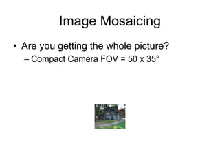
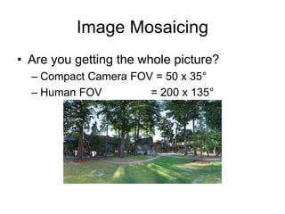
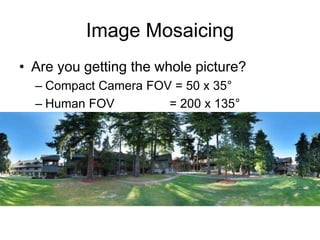
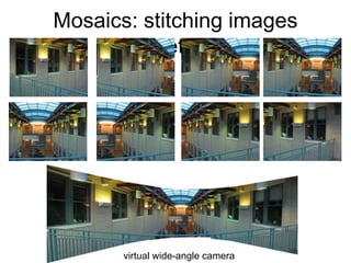
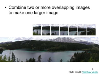
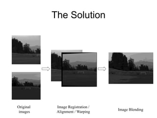
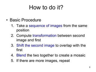
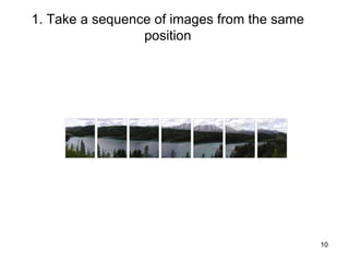
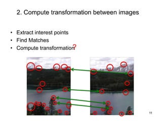
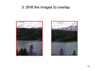
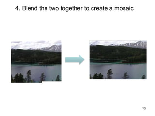
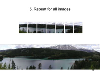
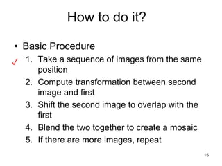
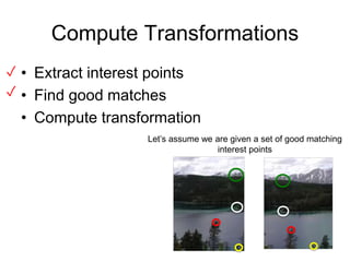
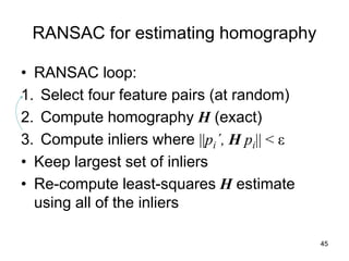
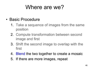
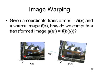
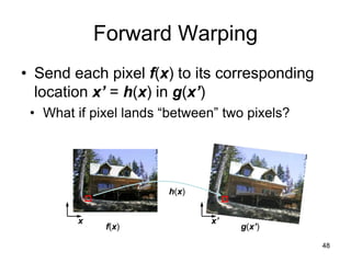
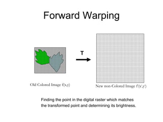
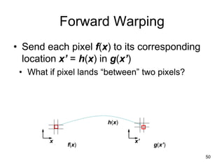
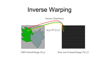
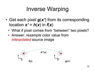
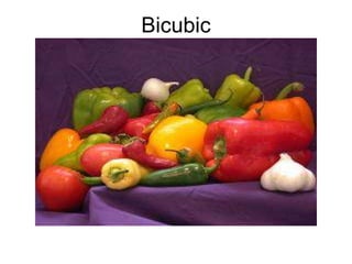
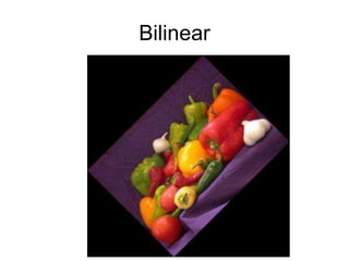
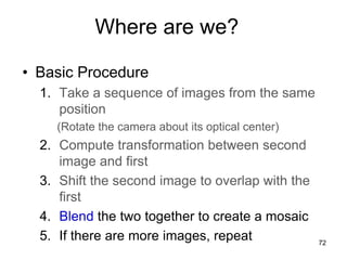
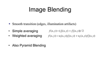
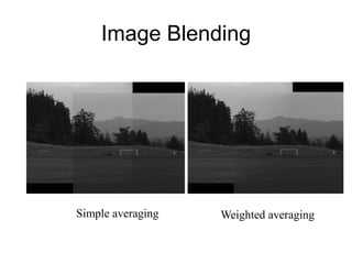
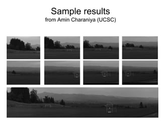
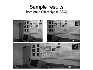
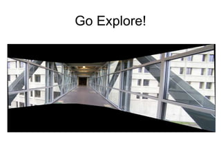
Image mosaicing involves stitching together multiple overlapping images to create a panoramic mosaic. The key steps are: 1) Taking a sequence of images from the same position and computing the transformation between each image, 2) Warping the images to align them by shifting pixels according to the transformation, and 3) Blending the aligned images together, with techniques like weighted averaging, to produce a seamless mosaic. Key challenges include dealing with moving objects, illumination variations, and interpolating pixel values when pixels are mapped between discrete pixel locations during warping.

1. Image Mosaicing
Elsayed Hemayed

2. Image Mosaicing
• Are you getting the whole picture?
– Compact Camera FOV = 50 x 35°

3. Image Mosaicing
• Are you getting the whole picture?
– Compact Camera FOV = 50 x 35°
– Human FOV = 200 x 135°

4. Image Mosaicing
• Are you getting the whole picture?
– Compact Camera FOV = 50 x 35°
– Human FOV = 200 x 135°
– Panoramic Mosaic = 360 x 180°

5. Mosaics: stitching images
together
virtual wide-angle camera

6. • Combine two or more overlapping images
to make one larger image
Add example
Slide credit: Vaibhav Vaish
6

7. The Problem
Q: “Static” ?
Ans.: No moving objects in the scene.
+Image 1 Image 2 Mosaiced image

8. The Solution
Original
images
Image Registration /
Alignment / Warping
Image Blending

9. How to do it?
• Basic Procedure
1. Take a sequence of images from the same
position
2. Compute transformation between second
image and first
3. Shift the second image to overlap with the
first
4. Blend the two together to create a mosaic
5. If there are more images, repeat
9

10. 1. Take a sequence of images from the same
position
10

11. 2. Compute transformation between images
• Extract interest points
• Find Matches
• Compute transformation?
11

12. 3. Shift the images to overlap
12

13. 4. Blend the two together to create a mosaic
13

14. 5. Repeat for all images
14

15. How to do it?
• Basic Procedure
1. Take a sequence of images from the same
position
2. Compute transformation between second
image and first
3. Shift the second image to overlap with the
first
4. Blend the two together to create a mosaic
5. If there are more images, repeat
✓
15

16. Compute Transformations
• Extract interest points
• Find good matches
• Compute transformation
✓
Let’s assume we are given a set of good matching
interest points
✓
16

17. Aligning images
Translations are not enough to align the images
left on top right on top

18. Image reprojection
• Observation
– Rather than thinking of this as a 3D reprojection,
think of it as a 2D image warp from one image to
another
18

19. Motion models
• What happens when we take two images
with a camera and try to align them?
• translation?
• rotation?
• scale?
• affine?
• Perspective?
19

20. Parametric (global) warping
• Examples of parametric warps:
translation rotation scaling
affine
perspective
20

21. 2D coordinate transformations
• translation: x’ = x + t x = (x,y)
• rotation: x’ = R x + t
• similarity: x’ = s R x + t
• affine: x’ = A x + t
• perspective: x’  H x x = (x,y,1)
(x is a homogeneous coordinate)
21

22. Translation
Preserves: Orientation

23. Translation and rotation

24. Scale

25. Similarity transformations
Similarity transform (4 DoF) = translation +
rotation + scale
Preserves: Angles

26. Shear

27. Affine transformations
Affine transform (6 DoF) = translation + rotation
+ scale + shear
Preserves: Parallelism

28. Projective transformations
a.k.a. Homographies
“keystone” distortions
Preserves: Straight Lines

29. Finding the transformation
Translation = 2 degrees of freedom
Similarity = 4 degrees of freedom
Affine = 6 degrees of freedom
Homography = 8 degrees of freedom
How many corresponding points do we
need to solve?

30. Solving for homographies
30
• A homography is a projective object, in that it has no
scale. It is represented by the above matrix, up to scale.
• One way of fixing the scale is to set one of the coordinates
to 1, though that choice is arbitrary.
• But that’s what most people do.

31. Solving for homographies
31

32. Solving for homographies
32
This is just for one pair of points.

33. Direct Linear Transforms (n points)
Defines a least squares problem:
• Since is only defined up to scale, solve for unit vector
• Solution: = eigenvector of with smallest
eigenvalue
• Works with 4 or more points
2n × 9 9 2n
33

34. 34
Matching features
What do we do about the “bad” matches?

35. Simple example: fit a line
• Rather than homography H (8 numbers)
fit y=ax+b (2 numbers a, b) to 2D pairs
35

36. Simple example: fit a line
• Pick 2 points
• Fit line
• Count inliers
36
3 inliers

37. Simple example: fit a line
• Pick 2 points
• Fit line
• Count inliers
37
4 inliers

38. Simple example: fit a line
• Pick 2 points
• Fit line
• Count inliers
38
9 inliers

39. Simple example: fit a line
• Pick 2 points
• Fit line
• Count inliers
39
8 inliers

40. Simple example: fit a line
• Use biggest set of inliers
• Do least-square fit
40

41. 41
RAndom SAmple Consensus
Select one match, count inliers

42. 42
RAndom SAmple Consensus
Select one match, count inliers

43. 43
Least squares fit (from inliers)
Find “average” translation vector

44. 44

45. RANSAC for estimating homography
• RANSAC loop:
1. Select four feature pairs (at random)
2. Compute homography H (exact)
3. Compute inliers where ||pi´, H pi|| < ε
• Keep largest set of inliers
• Re-compute least-squares H estimate
using all of the inliers
45

46. Where are we?
• Basic Procedure
1. Take a sequence of images from the same
position
2. Compute transformation between second
image and first
3. Shift the second image to overlap with the
first
4. Blend the two together to create a mosaic
5. If there are more images, repeat
46

47. Image Warping
• Given a coordinate transform x’ = h(x) and
a source image f(x), how do we compute a
transformed image g(x’) = f(h(x))?
f(x) g(x’)
x x’
h(x)
47

48. Forward Warping
• Send each pixel f(x) to its corresponding
location x’ = h(x) in g(x’)
f(x) g(x’)
x x’
h(x)
• What if pixel lands “between” two pixels?
48

49. Forward Warping
Old Colored Image f(x,y) New non-Colored Image f’(x’,y’)
T
Finding the point in the digital raster which matches
the transformed point and determining its brightness.

50. Forward Warping
• Send each pixel f(x) to its corresponding
location x’ = h(x) in g(x’)
f(x) g(x’)
x x’
h(x)
• What if pixel lands “between” two pixels?
50

51. 51
Inverse Warping
• Get each pixel g(x’) from its corresponding
location x’ = h(x) in f(x)
f(x) g(x’)
x x’
h-1(x)
• What if pixel comes from “between” two pixels?

52. Inverse Warping
Old Colored Image f(x,y) New non-Colored Image f’(x’,y’)
(x,y)=T-1(x’,y’)
Inverse Transform

53. 53
Inverse Warping
• Get each pixel g(x’) from its corresponding
location x’ = h(x) in f(x)
• What if pixel comes from “between” two pixels?
• Answer: resample color value from
interpolated source image
f(x) g(x’)
x x’
h-1(x)

54. Image Interpolation
• The brightness interpolation problem is usually
expressed in a dual way (by determining the
brightness of the original point in the input image
that corresponds to the point in the output image
lying on the discrete raster).
• Usually, a small neighborhood is used.

55. Nearest neighbor interpolation
Assigns to the point (x,y) the brightness value of
the nearest point g in the discrete raster
inverse planar
transformation of
the output image
onto the input
image

56. Linear Interpolation
Uses the four points neighboring the point
(x,y).

57. Interpolation vs. Nearest Neighbor
• Error of the nearest neighborhood
interpolation is at most half a pixel
• Linear interpolation can cause a small
decrease in resolution and blurring due to
its averaging nature.
• The problem of step like straight
boundaries with the nearest neighborhood
interpolation is reduced.

58. Interpolation Vs NN
NN
Interpolation

59. Bicubic Interpolation
• Improves the model of the brightness function by
approximating it locally by a bicubic polynomial
surface; sixteen neighboring points are used for
interpolation.
• The interpolation kernel (`Mexican hat') is given
by

60. Bicubic Interpolation
The brightness values of the
neighbors are first interpolated
horizontally to determine the
brightness values at the
locations outlined in red,
then
these values are interpolated
vertically to determine the
brightness at the target pixel
outlined in blue.
The summation goes from k-1 to
k+2 then from j-1 to j+2.

61. Implementation Steps
1. Determine the closest pixel to (x’,y’). Then select the
other 15 pixels (x-1 x+2 and y-1 y+2)
2. For Row 1 (y-1): Assume the four pixels have grey levels
(g1, g2, g3, g4) and are at distances dx (-1.1, -0.2, 0.9,
1.5).
Then the new grey level should be:
Gy-1=(4-8(1.1)+5(1.1^2)-(1.1^3))*g1 +
(4-8(1.5)+5(1.5^2)-(1.5^3))*g4 +
(1-2(0.2^2)+(0.2^3)*g2 +
(1-2(0.9^2)+(0.9^3)*g3.
3. Repeat for Gy, Gy+1, and Gy+2
4. Then Apply similar equation in step 2 but with the
calculated grey levels and dy (-1,0,1,2).

62. Bicubic Interpolation
• Bicubic interpolation does not suffer from the
step-like boundary problem of nearest
neighborhood interpolation, and copes with
linear interpolation blurring as well.
• Bicubic interpolation is often used in raster
displays that enable zooming with respect to an
arbitrary point -- if the nearest neighborhood
method were used, areas of the same
brightness would increase.
• Bicubic interpolation preserves fine details in the
image very well.
Cost !!

63. Nearest Neighbor

64. Bilinear Interpolation

65. Bicubic Interpolation

66. NN

67. Bilinear

68. Bicubic

69. NN

70. Bilinear

71. Bicubic

72. Where are we?
• Basic Procedure
1. Take a sequence of images from the same
position
(Rotate the camera about its optical center)
2. Compute transformation between second
image and first
3. Shift the second image to overlap with the
first
4. Blend the two together to create a mosaic
5. If there are more images, repeat 72

73. Image Blending
• Simple averaging
• Weighted averaging
• Also Pyramid Blending
2/)),('),((),( 21 yxfyxfyxf 
),('),(),(),(),( 2211 yxfyxwyxfyxwyxf 
 Smooth transition (edges, illumination artifacts)

74. Image Blending
Simple averaging Weighted averaging

75. Sample results
from Amin Charaniya (UCSC)

76. Sample results
from Amin Charaniya (UCSC)

77. Go Explore!