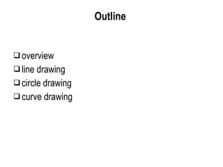
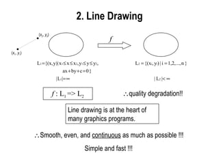
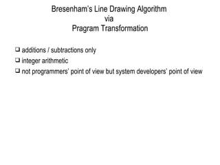
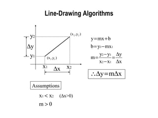
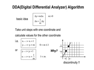
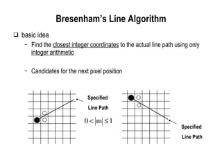
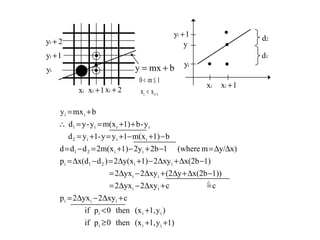
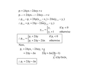
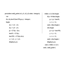
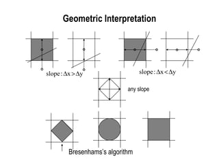
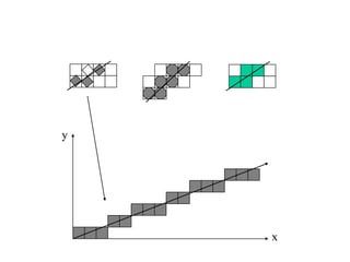
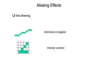
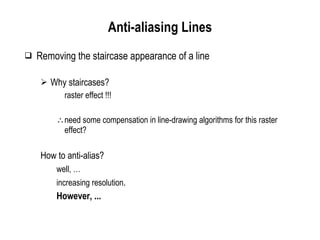
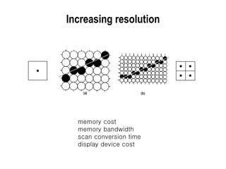
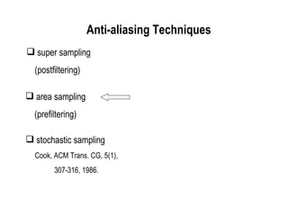
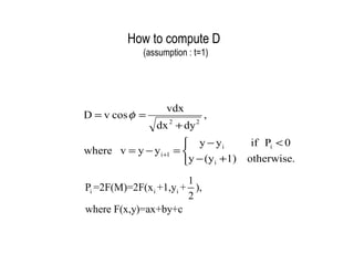
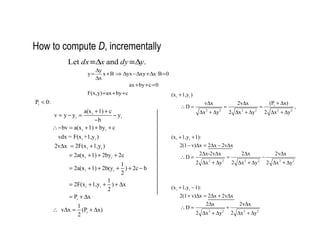
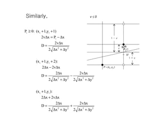
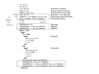
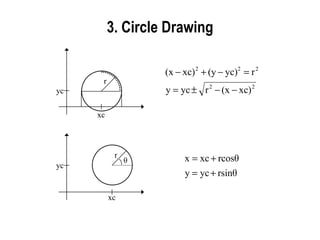
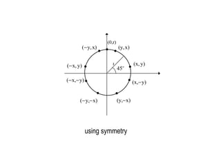
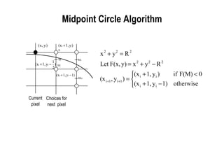
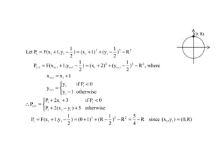
The document discusses techniques for line drawing and generalization in computer graphics. It covers Bresenham's line drawing algorithm, which uses only integer arithmetic for efficiency. It also discusses circle drawing using the midpoint circle algorithm and extensions to draw ellipses. Anti-aliasing techniques like area sampling are introduced to reduce jagged edges when rasterizing lines.

1. Line Drawing and Generalization Sung Yong Shin Dept. of Computer Science KAIST CS580 Computer Graphics

2. Outline overview line drawing circle drawing curve drawing

3. 1. Overview application data structures/models application programs graphics systems display devices graphics primitives OpenGL pixel information

4. Geometric Primitives Building blocks for a 3D object Application programs must describe their service requests to a graphics system using geometric primitives !!! points, lines, polygons Why not providing data structures directly to the graphics system?

5. display lists evaluators per-vertex operations & primitive assembly pixel operations rasterization texture assembly per-fragment operations OpenGL Rendering Pipeline per-vertex operations & primitive assembly rasterization frame buffer texture assembly display lists evaluators pixel operations per-fragment operations geometric data pixel data

6. Continuity 8-connectivity (king – continuity) 4-connectivity (rook – continuity)

7. 2. Line Drawing f f : L 1 => L 2  quality degradation!! Line drawing is at the heart of many graphics programs.  Smooth, even, and continuous as much as possible !!! Simple and fast !!! ( x 1 , y 1 ) ( x 2 , y 2 )

8. Bresenham’s Line Drawing Algorithm via Pragram Transformation additions / subtractions only integer arithmetic not programmers’ point of view but system developers’ point of view

9. var yt : real;  x,  y, xi, yi : integer; for xi := 0 to  x do begin yt := [  y/  x]*xi; yi := trunc(yt+[1/2]); display(xi,yi); end; var yt : real;  x,  y, xi, yi : integer; yt := 0; for xi := 0 to  x do begin yi := trunc(yt + [1/2]); display(xi,yi); yt := yt+[  y/  x] end; Eliminate multiplication !!!  x  y y = mx, m = [  y/  x] * **  x ≥  y ∴ m ≤ 1  x,  y: positive integers (0,0) ( ∆x, ∆y)

10. Motivation(Cont’) var ys : real;  x,  y, xi, yi : integer; ys := 1/2; for xi := 0 to dx do begin yi := trunc(ys); display(xi,yi); ys := ys+[  y/  x] end; var ysf : real;  x,  y, xi, ysi : integer; ysi := 0; ysf := 1/2; for xi := 0 to  x do begin display(xi,ysi); if ysf+[  y/  x] < 1 then begin ysf := ysf + [  y/  x]; end else begin ysi := ysi + 1; ysf := ysf + [  y/  x-1]; end; end; integer part fractional part *** ****

11. Motivation(Cont’) var  x,  y, xi, ysi, r : integer; ysi := 0; for xi := 0 to  x do begin display(xi,ysi); if then begin end else begin ysi := ysi + 1; end; end;

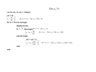
12. Motivation(Cont’) var  x,  y, xi, ysi, r : integer; ysi := 0; r := 2*  y -  x; for xi := 0 to  x do begin display(xi,ysi); if r < 0 then begin r := r + [2*  y]; end else begin ysi := ysi + 1; r := r + [2*  y -2*  x ]; end; end; Bresenham’s Algorithm !!! No multiplication/ division. No floating point operations.

13. Line-Drawing Algorithms Assumptions

14. DDA(Digital Differential Analyzer) Algorithm basic idea Take unit steps with one coordinate and calculate values for the other coordinate i.e. or discontinuity !! Why?

15. DDA(Cont’) procedure dda (x1, y1, x2, y2 : integer); var  x,  y, k : integer; x, y : real begin  x := x2 - x1;  y := y2 - y1; x := x1; y := y1; display(x,y); for k := 1 to  x do begin x := x + 1; y := y + [  y/  x]; display(round(x),round(y)); end { for k } end; { dda } expensive !! no *’s Assumption : 0  m <1, x1<x2

16. Bresenham’s Line Algorithm basic idea Find the closest integer coordinates to the actual line path using only integer arithmetic Candidates for the next pixel position Specified Line Path Specified Line Path

17. Bresenham’s Line algorithm(Cont’)

18. Bresenham’s Line algorithm(Cont’) =1

19. Bresenham’s Line algorithm(Cont’) procedure bres_line (x1, y1, x2, y2 : integer); var  x,  y, x,y,p,incrE,incrNE : integer; begin  x := x2 – x1;  y := y2 – y1; p := 2*  y -  x; incrE := 2*  y; incrNE := 2*(  y -  x); x := x1; y := y1; display(x,y); while x < x2 do begin if p<0 then begin p := p + incrE; x := x + 1; end; { then begin } else begin p := p + incrNE; y := y + 1; x := x + 1; end; { else begin } display (x, y); end { while x < x2 } end; { bres_line} Homework #2 Extend this algorithm for general cases.

20. Midpoint Line Algorithm Van Aken, “An Efficient Ellipse - Drawing Algorithm” IEEE CG & A, 4(9), 24-35, 1984. Current pixel Choices for next pixel

21. Midpoint Line Algorithm (Cont’)

22. Midpoint Line Alg. (Cont’)

23. Midpoint Line Alg. (Cont’) Midpoint Line Algorithm(Cont’) procedure mid_point (x1, y1, x2, y2,value : integer); var  x,  y,incrE,incrNE,p,x,y : integer; begin  x := x2 – x1;  y := y2 – y1; p := 2*  y -  x; incrE := 2*  y; incrNE := 2*(  y-  x); x := x1; y := y1; display(x,y); while x  x2 do begin if p < 0 then begin p := p + incrE; x := x + 1; end; { then begin } else begin p := p + incrNE; y := y + 1; x := x + 1; end; { else begin } display(x,y); end; { while x  x2 } end; { mid_point }

24. Geometric Interpretation any slope Bresenhams’s algorithm

25. Geometric Interpretation(Cont’) x y

26. Aliasing Effects staircases (or jaggies) intensity variation line drawing

27. animation texturing popping-up

28. Anti-aliasing Lines Removing the staircase appearance of a line Why staircases? raster effect !!! need some compensation in line-drawing algorithms for this raster effect? How to anti-alias? well, … increasing resolution . However, ...

29. Increasing resolution memory cost memory bandwidth scan conversion time display device cost

30. Anti-aliasing Line (Cont’) super sampling (postfiltering) area sampling (prefiltering) stochastic sampling Cook, ACM Trans. CG, 5(1), 307-316, 1986. Anti-aliasing Techniques

31. Area Sampling (Prefiltering)

32. Filters box filter cone filter unweighted area sampling weighted area sampling

33. Table look-up for f ( D , t ) The table is invariant of the slope of line! Why? The search key for the table is D! Why? D

34. Intensity Functions f ( D , t ) (assumption : t=1)

35. How to compute D (assumption : t=1)

36. How to compute D , incrementally

37. IF (Cont’) Similarly, M D 1 - v 1 + v v

38. IF (Cont’)  x := x2 - x1;  y := y2 - y1; p := 2 *  y -  x; {Initial value p 1 as before} incrE := 2 *  y; {Increment used for move to E} incrNE := 2 * (  y -  x); {Increment used for move to NE} two_v_  x := 0; {Numerator; v = 0 for start pixel} invDenom := 1 / (2 * Sqrt(  x *  x +  y *  y)); {Precomputed inverse denominator} two_  x_invDenom := 2 *  x * invDenom; {Precomputed constant} x := x1; y := y1; IntensifyPixel (x, y, 0); {Start pixel} IntensifyPixel(x, y + 1, two_  x_invDenom); {Neighbor} IntensifyPixel(x, y - 1, two_  x_invDenom); {Neighbor} while x < x2 do begin if p < 0 then begin {Choose E} two_v_  x := p +  x; p := p + incrE; x := x + 1 end else begin {Choose NE} two_v_  x := p -  x; p := p + incrNE; x := x + 1; y := y + 1; end ; {Now set chosen pixel and its neighbors} IntensifyPixel (x, y, two_v_  x * invDenom); IntensifyPixel (x, y + 1, two_  x_invDenom - two_v_  x * invDenom); IntensifyPixel (x, y - 1, two_  x_invDenom + two_v_  x * invDenom) end {while}

39. 3. Circle Drawing

40. symmetry using symmetry (0,r) r

41. Midpoint Circle Algorithm Current pixel Choices for next pixel

42. MCA (Cont’) (0, R)

43. MCA (Cont’)

44. MCA (Cont’) procedure MidpointCircle (radius,value : integer); var x,y : integer; P: real; begin x := 0; { initialization } y := radius; P := 5/4 - radius; CirclePoints(x,y,value); while y > x do begin if P < 0 then { select E } P : = P + 2*x + 3; x := x + 1; end else begin { select SE } P := P + 2*(x - y) + 5; x := x + 1; y := y - 1; end CirclePoints(x,y,value) end { while } end; { MidpointCircle } * ** d = P - 1/4 P = d + 1/4 * d = 1 - radius ** d < -1/4  d < 0 why? *** d := d + 2*x + 3 **** d := d + 2(x-y) + 5 *** **** (0, R) y=x

45. MCA (Cont’) procedure MidpointCircle (radius,value : integer); { Assumes center of circle is at origin. Integer arithmetic only } var x,y,d : integer; begin x := 0; { initialization } y := radius; d := 1 - radius; CirclePoints(x,y,value); while y > x do begin if d < 0 then { select E } d := d + 2*x + 3; x := x + 1; end else begin { select SE } d := d+2*(x - y) + 5; x := x + 1; y := y - 1; end CirclePoints(x,y,value) end { while } end; { MidpointCircle } Can you go further?

46. MCA (Cont’)

47. MCA (Cont’) procedure MidpointCircle (radius,value : integer); { This procedure uses second-order partial differences to compute increments in the decision variable. Assumes center of circle is origin. } var x,y,d,deltaE,deltaSE : integer; begin x := 0; { initialization } y := radius; d := 1 - radius; deltaE := 3; deltaSE := -2*radius + 5; CirclePoints(x,y,value); while y > x do begin if d < 0 then { select E } d := d + deltaE; deltaE := deltaE + 2; deltaSE := deltaSE + 2; x := x + 1; end else begin { select SE } d := d + deltaSE; deltaE := deltaE + 2; deltaSE := deltaSE + 4; x := x + 1; y := y - 1 end CirclePoints(x,y,value) end { while } end; { MidpointCircle }

48. Drawing Ellipse Homework #3 Modify the midpoint circle drawing algorithm to draw ellipses.

49. 4. Curve Drawing parametric equation discrete data set curve fitting piecewise linear