Download to read offline
![0 0 0 0 0 0 0 0 0 0
0 0 0 0 0 0 0 0 0 0
0 0 0 90 90 90 90 90 0 0
0 0 0 90 90 90 90 90 0 0
0 0 0 90 90 90 90 90 0 0
0 0 0 90 0 90 90 90 0 0
0 0 0 90 90 90 90 90 0 0
0 0 0 0 0 0 0 0 0 0
0 0 90 0 0 0 0 0 0 0
0 0 0 0 0 0 0 0 0 0
0
0 0 0 0 0 0 0 0 0 0
0 0 0 0 0 0 0 0 0 0
0 0 0 90 90 90 90 90 0 0
0 0 0 90 90 90 90 90 0 0
0 0 0 90 90 90 90 90 0 0
0 0 0 90 0 90 90 90 0 0
0 0 0 90 90 90 90 90 0 0
0 0 0 0 0 0 0 0 0 0
0 0 90 0 0 0 0 0 0 0
0 0 0 0 0 0 0 0 0 0
],[],[],[
,
lnkmflkgnmh
lk
[.,.]h[.,.]f
Noise removal using average filter
111
111
111
],[g
3](https://image.slidesharecdn.com/05cie552imageenhancement-200321060201/75/05-cie552-image_enhancement-3-2048.jpg)
![0 0 0 0 0 0 0 0 0 0
0 0 0 0 0 0 0 0 0 0
0 0 0 90 90 90 90 90 0 0
0 0 0 90 90 90 90 90 0 0
0 0 0 90 90 90 90 90 0 0
0 0 0 90 0 90 90 90 0 0
0 0 0 90 90 90 90 90 0 0
0 0 0 0 0 0 0 0 0 0
0 0 90 0 0 0 0 0 0 0
0 0 0 0 0 0 0 0 0 0
0 10
0 0 0 0 0 0 0 0 0 0
0 0 0 0 0 0 0 0 0 0
0 0 0 90 90 90 90 90 0 0
0 0 0 90 90 90 90 90 0 0
0 0 0 90 90 90 90 90 0 0
0 0 0 90 0 90 90 90 0 0
0 0 0 90 90 90 90 90 0 0
0 0 0 0 0 0 0 0 0 0
0 0 90 0 0 0 0 0 0 0
0 0 0 0 0 0 0 0 0 0
[.,.]h[.,.]f
111
111
111
],[g
],[],[],[
,
lnkmflkgnmh
lk
4](https://image.slidesharecdn.com/05cie552imageenhancement-200321060201/75/05-cie552-image_enhancement-4-2048.jpg)
![0 0 0 0 0 0 0 0 0 0
0 0 0 0 0 0 0 0 0 0
0 0 0 90 90 90 90 90 0 0
0 0 0 90 90 90 90 90 0 0
0 0 0 90 90 90 90 90 0 0
0 0 0 90 0 90 90 90 0 0
0 0 0 90 90 90 90 90 0 0
0 0 0 0 0 0 0 0 0 0
0 0 90 0 0 0 0 0 0 0
0 0 0 0 0 0 0 0 0 0
0 10 20
0 0 0 0 0 0 0 0 0 0
0 0 0 0 0 0 0 0 0 0
0 0 0 90 90 90 90 90 0 0
0 0 0 90 90 90 90 90 0 0
0 0 0 90 90 90 90 90 0 0
0 0 0 90 0 90 90 90 0 0
0 0 0 90 90 90 90 90 0 0
0 0 0 0 0 0 0 0 0 0
0 0 90 0 0 0 0 0 0 0
0 0 0 0 0 0 0 0 0 0
[.,.]h[.,.]f
111
111
111
],[g
],[],[],[
,
lnkmflkgnmh
lk
5](https://image.slidesharecdn.com/05cie552imageenhancement-200321060201/75/05-cie552-image_enhancement-5-2048.jpg)
![0 0 0 0 0 0 0 0 0 0
0 0 0 0 0 0 0 0 0 0
0 0 0 90 90 90 90 90 0 0
0 0 0 90 90 90 90 90 0 0
0 0 0 90 90 90 90 90 0 0
0 0 0 90 0 90 90 90 0 0
0 0 0 90 90 90 90 90 0 0
0 0 0 0 0 0 0 0 0 0
0 0 90 0 0 0 0 0 0 0
0 0 0 0 0 0 0 0 0 0
0 10 20 30
0 0 0 0 0 0 0 0 0 0
0 0 0 0 0 0 0 0 0 0
0 0 0 90 90 90 90 90 0 0
0 0 0 90 90 90 90 90 0 0
0 0 0 90 90 90 90 90 0 0
0 0 0 90 0 90 90 90 0 0
0 0 0 90 90 90 90 90 0 0
0 0 0 0 0 0 0 0 0 0
0 0 90 0 0 0 0 0 0 0
0 0 0 0 0 0 0 0 0 0
[.,.]h[.,.]f
111
111
111
],[g
],[],[],[
,
lnkmflkgnmh
lk
6](https://image.slidesharecdn.com/05cie552imageenhancement-200321060201/75/05-cie552-image_enhancement-6-2048.jpg)
![0 10 20 30 30
0 0 0 0 0 0 0 0 0 0
0 0 0 0 0 0 0 0 0 0
0 0 0 90 90 90 90 90 0 0
0 0 0 90 90 90 90 90 0 0
0 0 0 90 90 90 90 90 0 0
0 0 0 90 0 90 90 90 0 0
0 0 0 90 90 90 90 90 0 0
0 0 0 0 0 0 0 0 0 0
0 0 90 0 0 0 0 0 0 0
0 0 0 0 0 0 0 0 0 0
[.,.]h[.,.]f
111
111
111
],[g
],[],[],[
,
lnkmflkgnmh
lk
7](https://image.slidesharecdn.com/05cie552imageenhancement-200321060201/75/05-cie552-image_enhancement-7-2048.jpg)
![0 10 20 30 30
0 0 0 0 0 0 0 0 0 0
0 0 0 0 0 0 0 0 0 0
0 0 0 90 90 90 90 90 0 0
0 0 0 90 90 90 90 90 0 0
0 0 0 90 90 90 90 90 0 0
0 0 0 90 0 90 90 90 0 0
0 0 0 90 90 90 90 90 0 0
0 0 0 0 0 0 0 0 0 0
0 0 90 0 0 0 0 0 0 0
0 0 0 0 0 0 0 0 0 0
[.,.]h[.,.]f
111
111
111
],[g
?
],[],[],[
,
lnkmflkgnmh
lk
8](https://image.slidesharecdn.com/05cie552imageenhancement-200321060201/75/05-cie552-image_enhancement-8-2048.jpg)
![0 10 20 30 30
50
0 0 0 0 0 0 0 0 0 0
0 0 0 0 0 0 0 0 0 0
0 0 0 90 90 90 90 90 0 0
0 0 0 90 90 90 90 90 0 0
0 0 0 90 90 90 90 90 0 0
0 0 0 90 0 90 90 90 0 0
0 0 0 90 90 90 90 90 0 0
0 0 0 0 0 0 0 0 0 0
0 0 90 0 0 0 0 0 0 0
0 0 0 0 0 0 0 0 0 0
[.,.]h[.,.]f
111
111
111
],[g
?
],[],[],[
,
lnkmflkgnmh
lk
9](https://image.slidesharecdn.com/05cie552imageenhancement-200321060201/75/05-cie552-image_enhancement-9-2048.jpg)
![0 0 0 0 0 0 0 0 0 0
0 0 0 0 0 0 0 0 0 0
0 0 0 90 90 90 90 90 0 0
0 0 0 90 90 90 90 90 0 0
0 0 0 90 90 90 90 90 0 0
0 0 0 90 0 90 90 90 0 0
0 0 0 90 90 90 90 90 0 0
0 0 0 0 0 0 0 0 0 0
0 0 90 0 0 0 0 0 0 0
0 0 0 0 0 0 0 0 0 0
0 10 20 30 30 30 20 10
0 20 40 60 60 60 40 20
0 30 60 90 90 90 60 30
0 30 50 80 80 90 60 30
0 30 50 80 80 90 60 30
0 20 30 50 50 60 40 20
10 20 30 30 30 30 20 10
10 10 10 0 0 0 0 0
[.,.]h[.,.]f
111
111
111
],[g
],[],[],[
,
lnkmflkgnmh
lk
10](https://image.slidesharecdn.com/05cie552imageenhancement-200321060201/75/05-cie552-image_enhancement-10-2048.jpg)

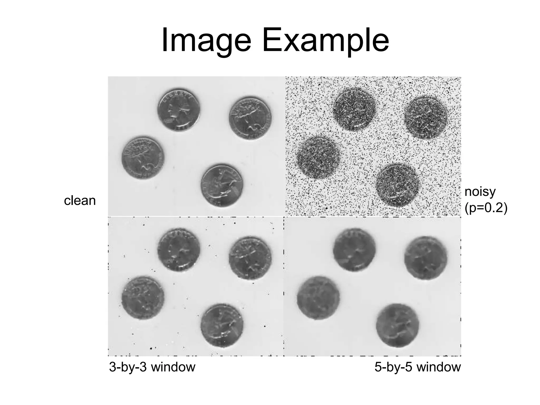
![Median Filter
• In a set of ordered values, the median is
the central value.
• The idea is to replace the current point in
the image by the median of the brightness
in its neighborhood
• It eliminate salt and pepper noise
Example ]56,55,54,255,52,0,50[y
54)( ymedian
]255,56,55,54,52,50,0[y
sorted](https://image.slidesharecdn.com/05cie552imageenhancement-200321060201/75/05-cie552-image_enhancement-12-2048.jpg)
![2D Numerical Example
225 225 225 226 226 226 226 226
225 225 255 226 226 226 225 226
226 226 225 226 0 226 226 255
255 226 225 0 226 226 226 226
225 255 0 225 226 226 226 255
255 225 224 226 226 0 225 226
226 225 225 226 255 226 226 228
226 226 225 226 226 226 226 226
0 225 225 226 226 226 226 226
225 225 226 226 226 226 226 226
225 226 226 226 226 226 226 226
226 226 225 225 226 226 226 226
225 225 225 225 226 226 226 226
225 225 225 226 226 226 226 226
225 225 225 226 226 226 226 226
226 226 226 226 226 226 226 226
Y X
^
Sorted: [0, 0, 0, 225, 225, 225, 226, 226, 226]](https://image.slidesharecdn.com/05cie552imageenhancement-200321060201/75/05-cie552-image_enhancement-13-2048.jpg)


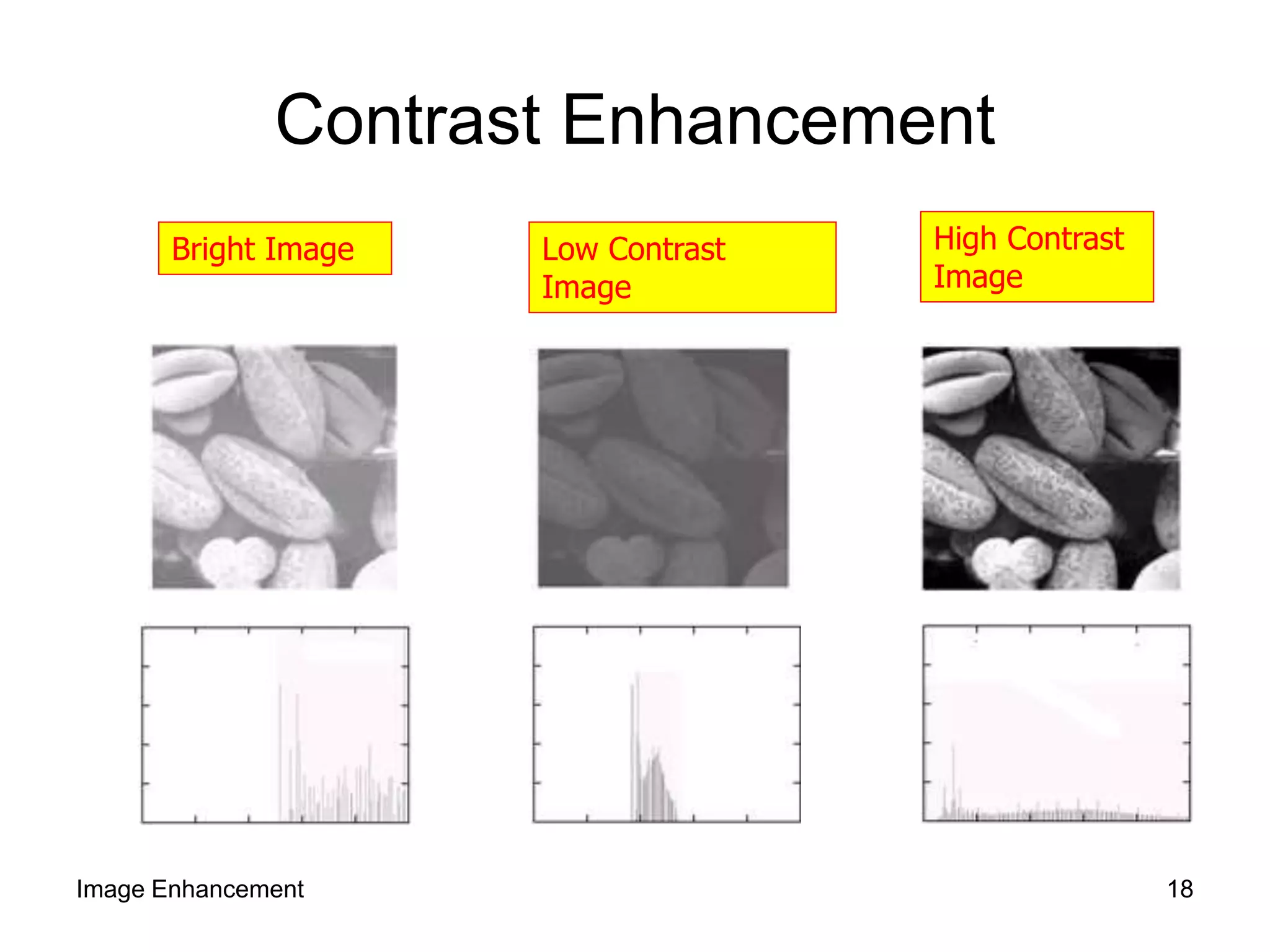


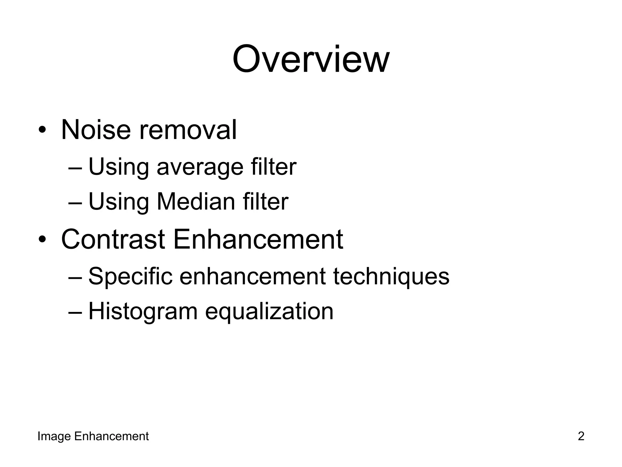
The document discusses image enhancement techniques for noise removal and contrast enhancement. It describes using average and median filters to remove noise, and histogram equalization to enhance contrast. Examples are provided to demonstrate noise removal using an average filter and median filter on sample images with added salt and pepper noise.