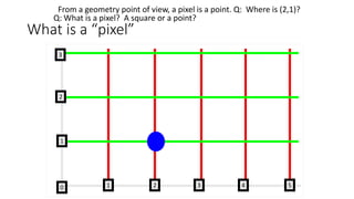
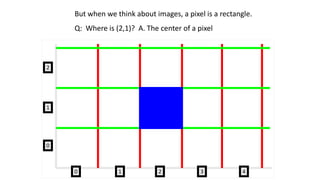
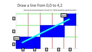
The document discusses computer graphics concepts like points, pixels, lines, and circles. It begins with definitions of pixels and how they relate to points in geometry. It then covers the basic structure for specifying points in OpenGL and how to draw points, lines, and triangles. Next, it discusses algorithms for drawing lines, including the digital differential analyzer (DDA) method and Bresenham's line algorithm. Finally, it covers circle drawing and introduces the mid-point circle algorithm. In summary:
1) It defines key computer graphics concepts like pixels, points, lines, and circles.
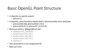
2) It explains the basic OpenGL functions for drawing points and lines and provides examples of drawing simple shapes.
3) It
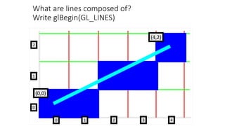
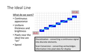
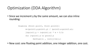
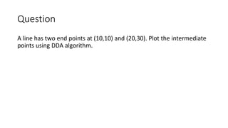
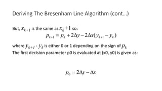
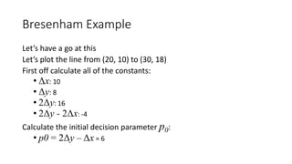
![Slope-Intercept Method
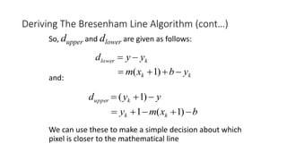
• From algebra: y = mx + b
• m = slope b = y intercept Let’s write some code
class Point
{
public:
int x, y;
int r,g,b;
};
unsigned byte framebuffer[IMAGE_WIDTH*IMAGE_HEIGHT*3];
DrawLine (Point point1, Point point2)
{
}](https://image.slidesharecdn.com/computergraphics2-200107084052/85/Computer-graphics-2-11-320.jpg)
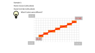
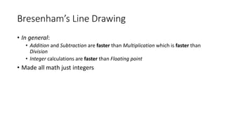
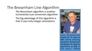
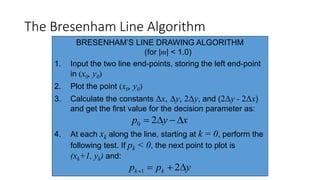
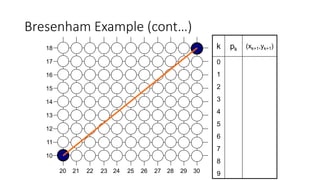
![Slope-Intercept Method
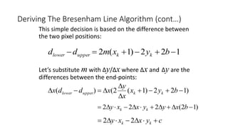
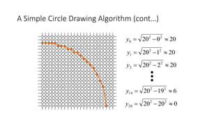
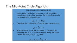
• From algebra: y = mx + b
• m = slope b = y intercept Let’s write some code
DrawLine (Point point1, Point point2){
m=(point2.y-point1.y) / (point2.x-point2.x);
b=point1.y + (-point1.x) * m;
for i=point1.x to point2.x
SetPixel(i , round(m*i+b)), pixel1.r, pixel1.g,
pixel1.b;}
SetPixel(int x, int y, int r, int g, int b){
framebuffer[(y * IMAGE_WIDTH+x) * 3 + 0]=r;
framebuffer[(y * IMAGE_WIDTH+x) * 3 + 1]=g;
framebuffer[(y * IMAGE_WIDTH+x) * 3 + 2]=b;}](https://image.slidesharecdn.com/computergraphics2-200107084052/85/Computer-graphics-2-12-320.jpg)
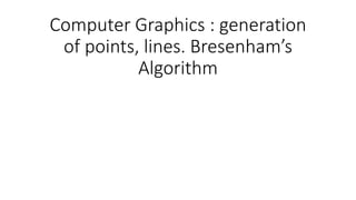
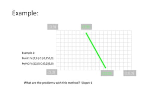
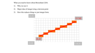
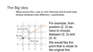
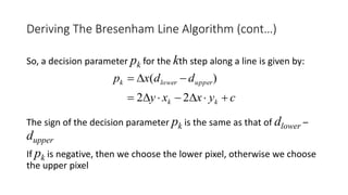
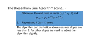
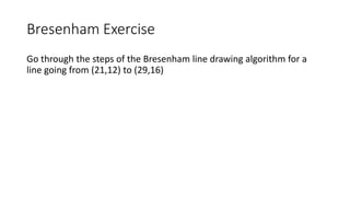
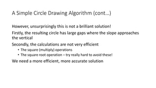
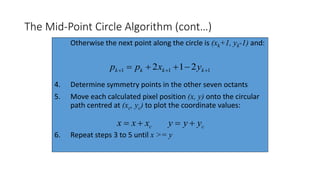
![How do we change the framebuffer?
(17,8)
(2,2)
(0,0) (18,0)
(0,9) What’s the index into GLubyte framebuffer[]? Point is 9,5](https://image.slidesharecdn.com/computergraphics2-200107084052/85/Computer-graphics-2-14-320.jpg)
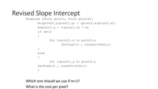
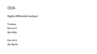
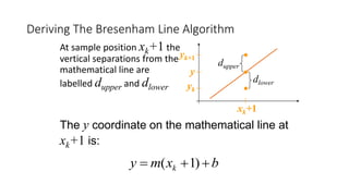
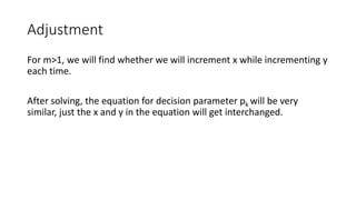
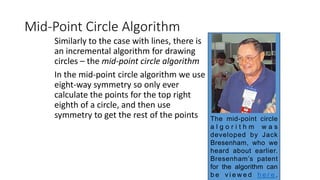
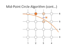
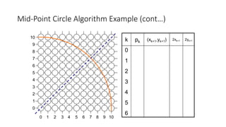
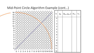
![Mid-Point Circle Algorithm (cont…)
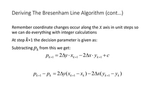
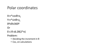
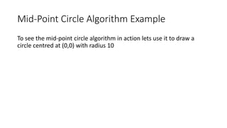
To ensure things are as efficient as possible we can do all of our calculations
incrementally
First consider:
or:
where yk+1 is either yk or yk-1 depending on the sign of pk
2
2
1
2
111
2
1]1)1[(
2
1,1
ryx
yxfp
kk
kkcirck
1)()()1(2 1
22
11 kkkkkkk yyyyxpp](https://image.slidesharecdn.com/computergraphics2-200107084052/85/Computer-graphics-2-49-320.jpg)


![Chapter 3 - Part 1 [Autosaved].pptx](https://cdn.slidesharecdn.com/ss_thumbnails/chapter3-part1autosaved-230109040832-9344385c-thumbnail.jpg?width=640&height=640&fit=bounds)