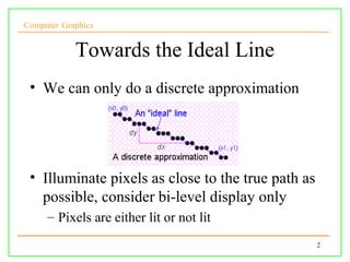
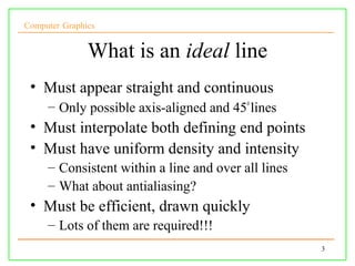
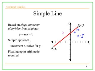
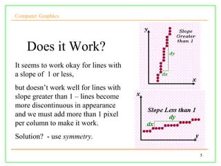
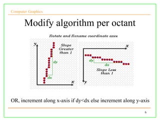
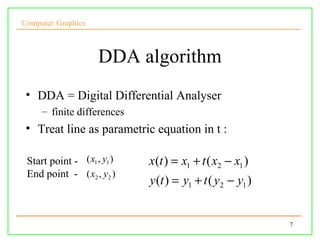
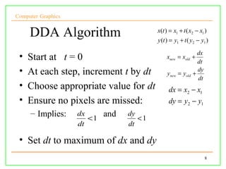
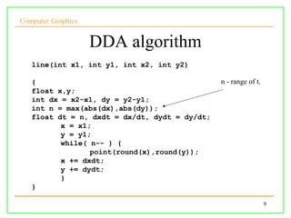
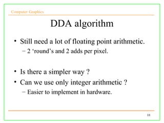
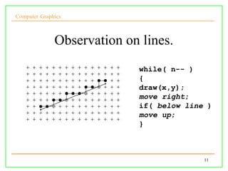
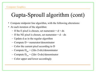
SlideShare a Scribd company logo
1 of 31
Computer Graphics


                Computer Graphics

                          Lecture 3
                    Line & Circle Drawing
Computer Graphics


            Towards the Ideal Line
 • We can only do a discrete approximation


 • Illuminate pixels as close to the true path as
   possible, consider bi-level display only
     – Pixels are either lit or not lit
                                                    2
Computer Graphics


               What is an ideal line
 • Must appear straight and continuous
     – Only possible axis-aligned and 45o lines
 • Must interpolate both defining end points
 • Must have uniform density and intensity
     – Consistent within a line and over all lines
     – What about antialiasing?
 • Must be efficient, drawn quickly
     – Lots of them are required!!!
                                                     3
Computer Graphics


                        Simple Line
 Based on slope-intercept
 algorithm from algebra:
           y = mx + b
 Simple approach:
   increment x, solve for y
 Floating point arithmetic
 required


                                      4
Computer Graphics


    Does it Work?
It seems to work okay for lines with
a slope of 1 or less,
but doesn’t work well for lines with
slope greater than 1 – lines become
more discontinuous in appearance
and we must add more than 1 pixel
per column to make it work.
Solution? - use symmetry.

                                       5
Computer Graphics


       Modify algorithm per octant


OR, increment along x-axis if dy<dx else increment along y-axis

                                                            6
Computer Graphics


                     DDA algorithm
 • DDA = Digital Differential Analyser
     – finite differences
 • Treat line as parametric equation in t :

 Start point - ( x1 , y1 )   x(t ) = x1 + t ( x2 − x1 )
 End point - ( x2 , y2 )
                             y (t ) = y1 + t ( y2 − y1 )


                                                           7
Computer Graphics


     DDA Algorithm                        x(t ) = x1 + t ( x2 − x1 )
                                          y (t ) = y1 + t ( y2 − y1 )

                                                               dx
 •   Start at t = 0                           xnew = xold +
                                                               dt
 •   At each step, increment t by dt           ynew = yold   +
                                                               dy
                                                               dt
 •   Choose appropriate value for dt           dx = x2 − x1
 •   Ensure no pixels are missed:              dy = y2 − y1
     – Implies:     dx      and   dy
                       <1            <1
                    dt            dt

 • Set dt to maximum of dx and dy
                                                                    8
Computer Graphics


                    DDA algorithm
   line(int x1, int y1, int x2, int y2)

   {                                           n - range of t.
   float x,y;
   int dx = x2-x1, dy = y2-y1;
   int n = max(abs(dx),abs(dy));
   float dt = n, dxdt = dx/dt, dydt = dy/dt;
          x = x1;
          y = y1;
          while( n-- ) {
                 point(round(x),round(y));
          x += dxdt;
          y += dydt;
          }
   }

                                                                 9
Computer Graphics


                    DDA algorithm
 • Still need a lot of floating point arithmetic.
     – 2 ‘round’s and 2 adds per pixel.


 • Is there a simpler way ?
 • Can we use only integer arithmetic ?
     – Easier to implement in hardware.


                                                    10
Computer Graphics


              Observation on lines.
                            while( n-- )
                            {
                            draw(x,y);
                            move right;
                            if( below line )
                            move up;
                            }


                                          11
Computer Graphics


      Testing for the side of a line.
 • Need a test to determine which side of a
   line a pixel lies.
 • Write the line in implicit form:
            F ( x, y ) = ax + by + c = 0
  •If (b<0) F<0 for points above the line, F>0 for
  points below.

                                                     12
Computer Graphics


      Testing for the side of a line.
                      F ( x, y ) = ax + by + c = 0
 • Need to find coefficients a,b,c.
 • Recall explicit, slope-intercept form :
                                          dy
                    y = mx + b and so y =    x+b
                                          dx

 • So:
             F ( x, y ) = dy.x − dx. y + c = 0
                                                     13
Computer Graphics

                    Decision variable.
    Let’s assume dy/dx < 0.5 (we can use symmetry)

    Evaluate F at point M                                      1
                                         d = F ( x p + 1, y p + )
                                                               2
    Referred to as decision variable


                                              NE


                                              M
                                              E

                            Previous   Choices for        Choices for
                              Pixel    Current pixel      Next pixel
                             (xp,yp)
Computer Graphics


                       Decision variable.
Evaluate d for next pixel, Depends on whether E or NE Is chosen :

If E chosen :
                            1                           1
d new   = F ( x p + 2, y p + ) = a ( x p + 2) + b( y p + ) + c
                            2                           2
                                                      But recall :
                                                                             1
                                                   d old = F ( x p + 1, y p + )
                          NE                                                 2
                                                                             1
                                    M              = a ( x p + 1) + b( y p + ) + c
                                                                             2
                           E
        Previous                    Choices for
                                                   So :
                                                              d new = d old + a
          Pixel     Choices for     Next pixel
         (xp,yp)    Current pixel                                     = d old + dy
                                                                                     15
Computer Graphics


                     Decision variable.
If NE was chosen :
                          3                           3
d new = F ( x p + 2, y p + ) = a ( x p + 2) + b( y p + ) + c
                          2                           2

                                M               So :
                      NE
                                              d new = d old + a + b
                      E
                                                       = d old + dy − dx
     Previous                   Choices for
       Pixel    Choices for     Next pixel
      (xp,yp)   Current pixel

                                                                           16
Computer Graphics


  Summary of mid-point algorithm
 • Choose between 2 pixels at each step based
   upon the sign of a decision variable.
 • Update the decision variable based upon
   which pixel is chosen.
 • Start point is simply first endpoint (x1,y1).
 • Need to calculate the initial value for d


                                               17
Computer Graphics


                     Initial value of d.
Start point is (x1,y1)
                                                            1                      1
                              d start   = F ( x1 + 1, y1 + ) = a( x1 + 1) + b( y1 + ) + c
                                                            2                      2
                                                                b
                                        = ax1 + by1 + c + a +
                                                                2
                                                              b
                                        = F ( x1 , y1 ) + a +
                                                              2

   But (x1,y1) is a point on the line, so F(x1,y1) =0

                         d start = dy − dx / 2
 Conventional to multiply by 2 to remove fraction ⇒ doesn’t effect sign.

                                                                                     18
Computer Graphics


                Midpoint algorithm
 void MidpointLine(int
   x1,y1,x2,y2)           while (x < x2) {
 {                               if (d<= 0) {
 int dx=x2-x1;                          d+=incrE;
                                        x++
 int dy=y2-y1;                  } else {
 int d=2*dy-dx;                        d+=incrNE;
                                       x++;
 int increE=2*dy;                      y++;
 int incrNE=2*(dy-dx);          }
                                WritePixel(x,y);
 x=x1;                    }
 y=y1;                    }

 WritePixel(x,y);

                                                    19
Computer Graphics


                    Circle drawing.
 • Can also use Bresenham to draw circles.

 • Use 8-fold symmetry                        E

                                                         M
                                               SE


                              Previous   Choices for     Choices for
                                Pixel    Current pixel   Next pixel


                                                               20
Computer Graphics


                    Circle drawing.
 • Implicit form for a circle is:
     f ( x, y ) = ( x − xc ) + ( y − yc ) − r
                                   2                      2   2


    If SE is chosen d new = d old + (2 x p − 2 y p + 5)
    If E is chosen d new = d old + (2 x p + 3)

  • Functions are linear equations in terms of (xp,yp)
      –Termed point of evaluation

                                                                  21
Computer Graphics


  Summary of line drawing so far.
 • Explicit form of line
     – Inefficient, difficult to control.
 • Parametric form of line.
     – Express line in terms of parameter t
     – DDA algorithm
 • Implicit form of line
     – Only need to test for ‘side’ of line.
     – Bresenham algorithm.
     – Can also draw circles.

                                               22
Computer Graphics


     Problems with Bresenham algorithm
 • Pixels are drawn as a single line ⇒ unequal
    line intensity with change in angle.


                      Pixel density = √2.n pixels/mm
                                             Can draw lines in darker colours
                                             according to line direction.
                                             -Better solution : antialiasing !
                                             -(eg. Gupta-Sproull algorithm)

         Pixel density = n pixels/mm
                                                                                 23
Computer Graphics


           Gupta-Sproull algorithm.
• Calculate the distance of the line and the pixel
  center
• Adjust the colour according to the distance
Computer Graphics


            Gupta-Sproull algorithm.
Calculate distance using features of mid-point algorithm
                                                             D = v cos φ
                                                                     vdx
                                                               =
                                                                   dx 2 + dy 2
                                                                                 dy
                                       NE
                                                                          dx

                                                     v     Angle = ∅
                                       M      D


                                      E

                                                                                 25
Computer Graphics

      Gupta-Sproull algorithm (cont)
Recall from the midpoint algorithm:
 F ( x, y ) = 2( ax + by + c ) = 0 (doubled to avoid fraction)          Line to draw
                                                                       NE
                                                       yp+1
So             y = ( ax + c )                                            m
                      −b                                           D          v
                                                  yp
                                                              xp         E    Θ
For pixel E:                                                           xp+1
      x p +1 = x p + 1        y p +1 = y p       v = y − y p +1

So:
                    a ( x p + 1) + c
              v=                       − yp
                          −b
Computer Graphics


   Gupta-Sproull algorithm (cont)
                                                                                    Line to draw
From previous slide:
                                                                                   NE
               a ( x p + 1) + c
          v=                      − yp                             yp+1
                     −b                                                              m
From the midpoint computation, y                               p
                                                                               D          v

                  b = − dx                                                xp         E    Θ
                                                                                   xp+1

So:
      vdx = a ( x p + 1) + by p + c = F ( x p + 1, y p ) / 2
Computer Graphics

        Gupta-Sproull algorithm (cont)
From the midpoint algorithm, we had the decision
 variable (remember?)
                                    1
    d = F ( M ) = F ( x p +1 , y p + )
                                    2                                 Line to draw
Going back to our previous equation:                                 NE
                                                     yp+1
  2vdx = F ( x p + 1, y p )                                            m

      = 2a ( x p + 1) + 2by p + 2c               py              D          v
                                                                            Θ
      = 2a ( x p + 1) + 2b( y p + 1 / 2) − 2b / 2 + 2c      xp         E
                                                                     xp+1
      = F ( x p + 1, y p + 1 / 2) − b
      = F (M ) − b
      = d −b
      = d + dx
Computer Graphics


      Gupta-Sproull algorithm (cont)
So,
                            d + dx
                    D=
                         2 dx 2 + dy 2

And the denominator is constant
Since we are blurring the line, we also need to
 compute the distances to points y p – 1 and yp + 1
            numerator for y p − 1 ⇒ 2(1 − v)dx = 2dx − 2vdx
            numerator for y p + 1 ⇒ 2(1 + v)dx = 2dx + 2vdx
Gupta-Sproull algorithm (cont)
Computer Graphics


If the NE pixel had been chosen:
             2vdx = F ( x p + 1, y p + 1)
                    = 2a( x p + 1) + 2(by p + 1) + 2c
                    = 2a( x p + 1) + 2b( y p + 1 / 2) + 2b / 2 + 2c
                    = F ( x p + 1, y p + 1 / 2) + b
                 = F (M ) + b
                 = d +b
                 = d − dx
          numerator for y p + 2 ⇒ 2(1 − v)dx = 2dx − 2vdx
          numerator for y p          ⇒ 2(1 + v)dx = 2dx + 2vdx
Computer Graphics


    Gupta-Sproull algorithm (cont)
 • Compute midpoint line algorithm, with the following alterations:
 • At each iteration of the algorithm:
    – If the E pixel is chosen, set numerator = d + dx
    – If the NE pixel is chosen, set numerator = d – dx
    – Update d as in the regular algorithm
    – Compute D = numerator/denominator
    – Color the current pixel according to D
    – Compute Dupper = (2dx-2vdx)/denominator
    – Compute Dlower = (2dx+2vdx)/denominator
    – Color upper and lower accordingly

More Related Content

What's hot

Neural Networks: Principal Component Analysis (PCA)
Neural Networks: Principal Component Analysis (PCA)Neural Networks: Principal Component Analysis (PCA)
Neural Networks: Principal Component Analysis (PCA)Mostafa G. M. Mostafa
 
AI Heuristic Search - Beam Search - Simulated Annealing
AI Heuristic Search - Beam Search - Simulated AnnealingAI Heuristic Search - Beam Search - Simulated Annealing
AI Heuristic Search - Beam Search - Simulated AnnealingAhmed Gad
 
Machine Learning and Real-World Applications
Machine Learning and Real-World ApplicationsMachine Learning and Real-World Applications
Machine Learning and Real-World ApplicationsMachinePulse
 
AI simple search strategies
AI simple search strategiesAI simple search strategies
AI simple search strategiesRenas Rekany
 
backpropagation in neural networks
backpropagation in neural networksbackpropagation in neural networks
backpropagation in neural networksAkash Goel
 
pattern classification
pattern classificationpattern classification
pattern classificationRanjan Ganguli
 
Hand Gesture Recognition using Neural Network
Hand Gesture Recognition using Neural NetworkHand Gesture Recognition using Neural Network
Hand Gesture Recognition using Neural NetworkBhagwat Singh Rathore
 
Amazon Product Review Sentiment Analysis with Machine Learning
Amazon Product Review Sentiment Analysis with Machine LearningAmazon Product Review Sentiment Analysis with Machine Learning
Amazon Product Review Sentiment Analysis with Machine Learningijtsrd
 
Intelligent mobile Robotics & Perception SystemsIntelligent mobile Robotics ...
Intelligent mobile Robotics  & Perception SystemsIntelligent mobile Robotics ...Intelligent mobile Robotics  & Perception SystemsIntelligent mobile Robotics ...
Intelligent mobile Robotics & Perception SystemsIntelligent mobile Robotics ...Gouasmia Zakaria
 
k Nearest Neighbor
k Nearest Neighbork Nearest Neighbor
k Nearest Neighborbutest
 

What's hot (20)

Physical symbol system
Physical symbol systemPhysical symbol system
Physical symbol system
 
Neural Networks: Principal Component Analysis (PCA)
Neural Networks: Principal Component Analysis (PCA)Neural Networks: Principal Component Analysis (PCA)
Neural Networks: Principal Component Analysis (PCA)
 
AI_Unit I notes .pdf
AI_Unit I notes .pdfAI_Unit I notes .pdf
AI_Unit I notes .pdf
 
AI Heuristic Search - Beam Search - Simulated Annealing
AI Heuristic Search - Beam Search - Simulated AnnealingAI Heuristic Search - Beam Search - Simulated Annealing
AI Heuristic Search - Beam Search - Simulated Annealing
 
Agents1
Agents1Agents1
Agents1
 
PPT.pptx
PPT.pptxPPT.pptx
PPT.pptx
 
Machine Learning and Real-World Applications
Machine Learning and Real-World ApplicationsMachine Learning and Real-World Applications
Machine Learning and Real-World Applications
 
Hand Gesture recognition
Hand Gesture recognitionHand Gesture recognition
Hand Gesture recognition
 
AI simple search strategies
AI simple search strategiesAI simple search strategies
AI simple search strategies
 
AI
AIAI
AI
 
Kapil dikshit ppt
Kapil dikshit pptKapil dikshit ppt
Kapil dikshit ppt
 
backpropagation in neural networks
backpropagation in neural networksbackpropagation in neural networks
backpropagation in neural networks
 
Cosc 208 lecture note-1
Cosc 208 lecture note-1Cosc 208 lecture note-1
Cosc 208 lecture note-1
 
AI: AI & Problem Solving
AI: AI & Problem SolvingAI: AI & Problem Solving
AI: AI & Problem Solving
 
pattern classification
pattern classificationpattern classification
pattern classification
 
Hand Gesture Recognition using Neural Network
Hand Gesture Recognition using Neural NetworkHand Gesture Recognition using Neural Network
Hand Gesture Recognition using Neural Network
 
Amazon Product Review Sentiment Analysis with Machine Learning
Amazon Product Review Sentiment Analysis with Machine LearningAmazon Product Review Sentiment Analysis with Machine Learning
Amazon Product Review Sentiment Analysis with Machine Learning
 
Intelligent mobile Robotics & Perception SystemsIntelligent mobile Robotics ...
Intelligent mobile Robotics  & Perception SystemsIntelligent mobile Robotics ...Intelligent mobile Robotics  & Perception SystemsIntelligent mobile Robotics ...
Intelligent mobile Robotics & Perception SystemsIntelligent mobile Robotics ...
 
k Nearest Neighbor
k Nearest Neighbork Nearest Neighbor
k Nearest Neighbor
 
Game playing in AI
Game playing in AIGame playing in AI
Game playing in AI
 

Similar to Lect3cg2011

Emat 213 study guide
Emat 213 study guideEmat 213 study guide
Emat 213 study guideakabaka12
 
23 industrial engineering
23 industrial engineering23 industrial engineering
23 industrial engineeringmloeb825
 
Scientific Computing with Python Webinar 9/18/2009:Curve Fitting
Scientific Computing with Python Webinar 9/18/2009:Curve FittingScientific Computing with Python Webinar 9/18/2009:Curve Fitting
Scientific Computing with Python Webinar 9/18/2009:Curve FittingEnthought, Inc.
 
Kernel based models for geo- and environmental sciences- Alexei Pozdnoukhov –...
Kernel based models for geo- and environmental sciences- Alexei Pozdnoukhov –...Kernel based models for geo- and environmental sciences- Alexei Pozdnoukhov –...
Kernel based models for geo- and environmental sciences- Alexei Pozdnoukhov –...Beniamino Murgante
 
Open GL T0074 56 sm4
Open GL T0074 56 sm4Open GL T0074 56 sm4
Open GL T0074 56 sm4Roziq Bahtiar
 
Line drawing Algorithm DDA in computer Graphics.pdf
Line drawing Algorithm DDA in computer Graphics.pdfLine drawing Algorithm DDA in computer Graphics.pdf
Line drawing Algorithm DDA in computer Graphics.pdfRAJARATNAS
 
Output Primitives in Computer Graphics and Multimedia
Output Primitives in Computer Graphics and MultimediaOutput Primitives in Computer Graphics and Multimedia
Output Primitives in Computer Graphics and Multimediasaranyan75
 
Computer Graphics and Multimedia Output primitives
Computer Graphics and Multimedia Output primitivesComputer Graphics and Multimedia Output primitives
Computer Graphics and Multimedia Output primitivessaranyan75
 
Computer Aided Manufacturing Design
Computer Aided Manufacturing DesignComputer Aided Manufacturing Design
Computer Aided Manufacturing DesignV Tripathi
 
chapter 3 , foley.pptxhuujjjjjjjkjmmmm. Ibibhvucufucuvivihohi
chapter 3 , foley.pptxhuujjjjjjjkjmmmm.  Ibibhvucufucuvivihohichapter 3 , foley.pptxhuujjjjjjjkjmmmm.  Ibibhvucufucuvivihohi
chapter 3 , foley.pptxhuujjjjjjjkjmmmm. Ibibhvucufucuvivihohi54MahakBansal
 
Mid point line Algorithm - Computer Graphics
Mid point line Algorithm - Computer GraphicsMid point line Algorithm - Computer Graphics
Mid point line Algorithm - Computer GraphicsDrishti Bhalla
 
Digital differential analyzer
Digital differential analyzerDigital differential analyzer
Digital differential analyzerSajid Hasan
 
Integral table
Integral tableIntegral table
Integral tablebags07
 

Similar to Lect3cg2011 (20)

Assignment6
Assignment6Assignment6
Assignment6
 
Emat 213 study guide
Emat 213 study guideEmat 213 study guide
Emat 213 study guide
 
23 industrial engineering
23 industrial engineering23 industrial engineering
23 industrial engineering
 
Scientific Computing with Python Webinar 9/18/2009:Curve Fitting
Scientific Computing with Python Webinar 9/18/2009:Curve FittingScientific Computing with Python Webinar 9/18/2009:Curve Fitting
Scientific Computing with Python Webinar 9/18/2009:Curve Fitting
 
Kernel based models for geo- and environmental sciences- Alexei Pozdnoukhov –...
Kernel based models for geo- and environmental sciences- Alexei Pozdnoukhov –...Kernel based models for geo- and environmental sciences- Alexei Pozdnoukhov –...
Kernel based models for geo- and environmental sciences- Alexei Pozdnoukhov –...
 
Open GL T0074 56 sm4
Open GL T0074 56 sm4Open GL T0074 56 sm4
Open GL T0074 56 sm4
 
Line drawing Algorithm DDA in computer Graphics.pdf
Line drawing Algorithm DDA in computer Graphics.pdfLine drawing Algorithm DDA in computer Graphics.pdf
Line drawing Algorithm DDA in computer Graphics.pdf
 
Line circle draw
Line circle drawLine circle draw
Line circle draw
 
raster algorithm.pdf
raster algorithm.pdfraster algorithm.pdf
raster algorithm.pdf
 
Sect1 4
Sect1 4Sect1 4
Sect1 4
 
Output Primitives in Computer Graphics and Multimedia
Output Primitives in Computer Graphics and MultimediaOutput Primitives in Computer Graphics and Multimedia
Output Primitives in Computer Graphics and Multimedia
 
Computer Graphics and Multimedia Output primitives
Computer Graphics and Multimedia Output primitivesComputer Graphics and Multimedia Output primitives
Computer Graphics and Multimedia Output primitives
 
Computer Aided Manufacturing Design
Computer Aided Manufacturing DesignComputer Aided Manufacturing Design
Computer Aided Manufacturing Design
 
Computer graphics
Computer graphics   Computer graphics
Computer graphics
 
Computer graphics
Computer graphics   Computer graphics
Computer graphics
 
chapter 3 , foley.pptxhuujjjjjjjkjmmmm. Ibibhvucufucuvivihohi
chapter 3 , foley.pptxhuujjjjjjjkjmmmm.  Ibibhvucufucuvivihohichapter 3 , foley.pptxhuujjjjjjjkjmmmm.  Ibibhvucufucuvivihohi
chapter 3 , foley.pptxhuujjjjjjjkjmmmm. Ibibhvucufucuvivihohi
 
Mid point line Algorithm - Computer Graphics
Mid point line Algorithm - Computer GraphicsMid point line Algorithm - Computer Graphics
Mid point line Algorithm - Computer Graphics
 
Digital differential analyzer
Digital differential analyzerDigital differential analyzer
Digital differential analyzer
 
Cs 601
Cs 601Cs 601
Cs 601
 
Integral table
Integral tableIntegral table
Integral table
 

Lect3cg2011

  • 1. Computer Graphics Computer Graphics Lecture 3 Line & Circle Drawing
  • 2. Computer Graphics Towards the Ideal Line • We can only do a discrete approximation • Illuminate pixels as close to the true path as possible, consider bi-level display only – Pixels are either lit or not lit 2
  • 3. Computer Graphics What is an ideal line • Must appear straight and continuous – Only possible axis-aligned and 45o lines • Must interpolate both defining end points • Must have uniform density and intensity – Consistent within a line and over all lines – What about antialiasing? • Must be efficient, drawn quickly – Lots of them are required!!! 3
  • 4. Computer Graphics Simple Line Based on slope-intercept algorithm from algebra: y = mx + b Simple approach: increment x, solve for y Floating point arithmetic required 4
  • 5. Computer Graphics Does it Work? It seems to work okay for lines with a slope of 1 or less, but doesn’t work well for lines with slope greater than 1 – lines become more discontinuous in appearance and we must add more than 1 pixel per column to make it work. Solution? - use symmetry. 5
  • 6. Computer Graphics Modify algorithm per octant OR, increment along x-axis if dy<dx else increment along y-axis 6
  • 7. Computer Graphics DDA algorithm • DDA = Digital Differential Analyser – finite differences • Treat line as parametric equation in t : Start point - ( x1 , y1 ) x(t ) = x1 + t ( x2 − x1 ) End point - ( x2 , y2 ) y (t ) = y1 + t ( y2 − y1 ) 7
  • 8. Computer Graphics DDA Algorithm x(t ) = x1 + t ( x2 − x1 ) y (t ) = y1 + t ( y2 − y1 ) dx • Start at t = 0 xnew = xold + dt • At each step, increment t by dt ynew = yold + dy dt • Choose appropriate value for dt dx = x2 − x1 • Ensure no pixels are missed: dy = y2 − y1 – Implies: dx and dy <1 <1 dt dt • Set dt to maximum of dx and dy 8
  • 9. Computer Graphics DDA algorithm line(int x1, int y1, int x2, int y2) { n - range of t. float x,y; int dx = x2-x1, dy = y2-y1; int n = max(abs(dx),abs(dy)); float dt = n, dxdt = dx/dt, dydt = dy/dt; x = x1; y = y1; while( n-- ) { point(round(x),round(y)); x += dxdt; y += dydt; } } 9
  • 10. Computer Graphics DDA algorithm • Still need a lot of floating point arithmetic. – 2 ‘round’s and 2 adds per pixel. • Is there a simpler way ? • Can we use only integer arithmetic ? – Easier to implement in hardware. 10
  • 11. Computer Graphics Observation on lines. while( n-- ) { draw(x,y); move right; if( below line ) move up; } 11
  • 12. Computer Graphics Testing for the side of a line. • Need a test to determine which side of a line a pixel lies. • Write the line in implicit form: F ( x, y ) = ax + by + c = 0 •If (b<0) F<0 for points above the line, F>0 for points below. 12
  • 13. Computer Graphics Testing for the side of a line. F ( x, y ) = ax + by + c = 0 • Need to find coefficients a,b,c. • Recall explicit, slope-intercept form : dy y = mx + b and so y = x+b dx • So: F ( x, y ) = dy.x − dx. y + c = 0 13
  • 14. Computer Graphics Decision variable. Let’s assume dy/dx < 0.5 (we can use symmetry) Evaluate F at point M 1 d = F ( x p + 1, y p + ) 2 Referred to as decision variable NE M E Previous Choices for Choices for Pixel Current pixel Next pixel (xp,yp)
  • 15. Computer Graphics Decision variable. Evaluate d for next pixel, Depends on whether E or NE Is chosen : If E chosen : 1 1 d new = F ( x p + 2, y p + ) = a ( x p + 2) + b( y p + ) + c 2 2 But recall : 1 d old = F ( x p + 1, y p + ) NE 2 1 M = a ( x p + 1) + b( y p + ) + c 2 E Previous Choices for So : d new = d old + a Pixel Choices for Next pixel (xp,yp) Current pixel = d old + dy 15
  • 16. Computer Graphics Decision variable. If NE was chosen : 3 3 d new = F ( x p + 2, y p + ) = a ( x p + 2) + b( y p + ) + c 2 2 M So : NE d new = d old + a + b E = d old + dy − dx Previous Choices for Pixel Choices for Next pixel (xp,yp) Current pixel 16
  • 17. Computer Graphics Summary of mid-point algorithm • Choose between 2 pixels at each step based upon the sign of a decision variable. • Update the decision variable based upon which pixel is chosen. • Start point is simply first endpoint (x1,y1). • Need to calculate the initial value for d 17
  • 18. Computer Graphics Initial value of d. Start point is (x1,y1) 1 1 d start = F ( x1 + 1, y1 + ) = a( x1 + 1) + b( y1 + ) + c 2 2 b = ax1 + by1 + c + a + 2 b = F ( x1 , y1 ) + a + 2 But (x1,y1) is a point on the line, so F(x1,y1) =0 d start = dy − dx / 2 Conventional to multiply by 2 to remove fraction ⇒ doesn’t effect sign. 18
  • 19. Computer Graphics Midpoint algorithm void MidpointLine(int x1,y1,x2,y2) while (x < x2) { { if (d<= 0) { int dx=x2-x1; d+=incrE; x++ int dy=y2-y1; } else { int d=2*dy-dx; d+=incrNE; x++; int increE=2*dy; y++; int incrNE=2*(dy-dx); } WritePixel(x,y); x=x1; } y=y1; } WritePixel(x,y); 19
  • 20. Computer Graphics Circle drawing. • Can also use Bresenham to draw circles. • Use 8-fold symmetry E M SE Previous Choices for Choices for Pixel Current pixel Next pixel 20
  • 21. Computer Graphics Circle drawing. • Implicit form for a circle is: f ( x, y ) = ( x − xc ) + ( y − yc ) − r 2 2 2 If SE is chosen d new = d old + (2 x p − 2 y p + 5) If E is chosen d new = d old + (2 x p + 3) • Functions are linear equations in terms of (xp,yp) –Termed point of evaluation 21
  • 22. Computer Graphics Summary of line drawing so far. • Explicit form of line – Inefficient, difficult to control. • Parametric form of line. – Express line in terms of parameter t – DDA algorithm • Implicit form of line – Only need to test for ‘side’ of line. – Bresenham algorithm. – Can also draw circles. 22
  • 23. Computer Graphics Problems with Bresenham algorithm • Pixels are drawn as a single line ⇒ unequal line intensity with change in angle. Pixel density = √2.n pixels/mm Can draw lines in darker colours according to line direction. -Better solution : antialiasing ! -(eg. Gupta-Sproull algorithm) Pixel density = n pixels/mm 23
  • 24. Computer Graphics Gupta-Sproull algorithm. • Calculate the distance of the line and the pixel center • Adjust the colour according to the distance
  • 25. Computer Graphics Gupta-Sproull algorithm. Calculate distance using features of mid-point algorithm D = v cos φ vdx = dx 2 + dy 2 dy NE dx v Angle = ∅ M D E 25
  • 26. Computer Graphics Gupta-Sproull algorithm (cont) Recall from the midpoint algorithm: F ( x, y ) = 2( ax + by + c ) = 0 (doubled to avoid fraction) Line to draw NE yp+1 So y = ( ax + c ) m −b D v yp xp E Θ For pixel E: xp+1 x p +1 = x p + 1 y p +1 = y p v = y − y p +1 So: a ( x p + 1) + c v= − yp −b
  • 27. Computer Graphics Gupta-Sproull algorithm (cont) Line to draw From previous slide: NE a ( x p + 1) + c v= − yp yp+1 −b m From the midpoint computation, y p D v b = − dx xp E Θ xp+1 So: vdx = a ( x p + 1) + by p + c = F ( x p + 1, y p ) / 2
  • 28. Computer Graphics Gupta-Sproull algorithm (cont) From the midpoint algorithm, we had the decision variable (remember?) 1 d = F ( M ) = F ( x p +1 , y p + ) 2 Line to draw Going back to our previous equation: NE yp+1 2vdx = F ( x p + 1, y p ) m = 2a ( x p + 1) + 2by p + 2c py D v Θ = 2a ( x p + 1) + 2b( y p + 1 / 2) − 2b / 2 + 2c xp E xp+1 = F ( x p + 1, y p + 1 / 2) − b = F (M ) − b = d −b = d + dx
  • 29. Computer Graphics Gupta-Sproull algorithm (cont) So, d + dx D= 2 dx 2 + dy 2 And the denominator is constant Since we are blurring the line, we also need to compute the distances to points y p – 1 and yp + 1 numerator for y p − 1 ⇒ 2(1 − v)dx = 2dx − 2vdx numerator for y p + 1 ⇒ 2(1 + v)dx = 2dx + 2vdx
  • 30. Gupta-Sproull algorithm (cont) Computer Graphics If the NE pixel had been chosen: 2vdx = F ( x p + 1, y p + 1) = 2a( x p + 1) + 2(by p + 1) + 2c = 2a( x p + 1) + 2b( y p + 1 / 2) + 2b / 2 + 2c = F ( x p + 1, y p + 1 / 2) + b = F (M ) + b = d +b = d − dx numerator for y p + 2 ⇒ 2(1 − v)dx = 2dx − 2vdx numerator for y p ⇒ 2(1 + v)dx = 2dx + 2vdx
  • 31. Computer Graphics Gupta-Sproull algorithm (cont) • Compute midpoint line algorithm, with the following alterations: • At each iteration of the algorithm: – If the E pixel is chosen, set numerator = d + dx – If the NE pixel is chosen, set numerator = d – dx – Update d as in the regular algorithm – Compute D = numerator/denominator – Color the current pixel according to D – Compute Dupper = (2dx-2vdx)/denominator – Compute Dlower = (2dx+2vdx)/denominator – Color upper and lower accordingly

Editor's Notes

  1. Important algorithm.
  2. Very important.
  3. Only principle of this method important.