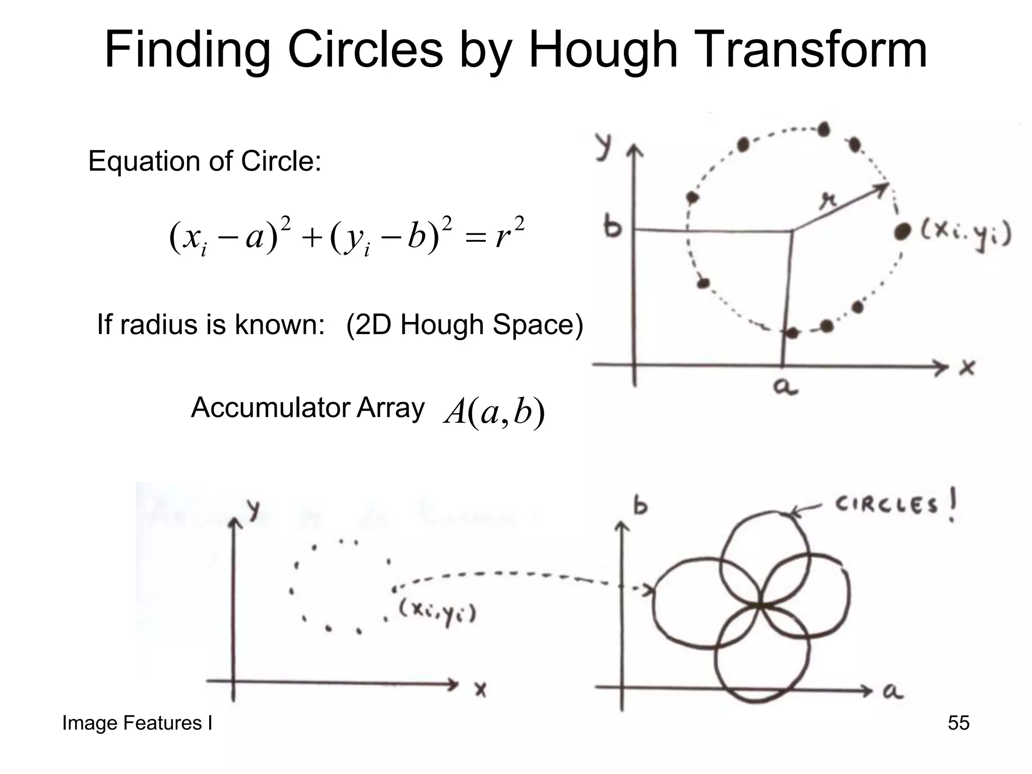
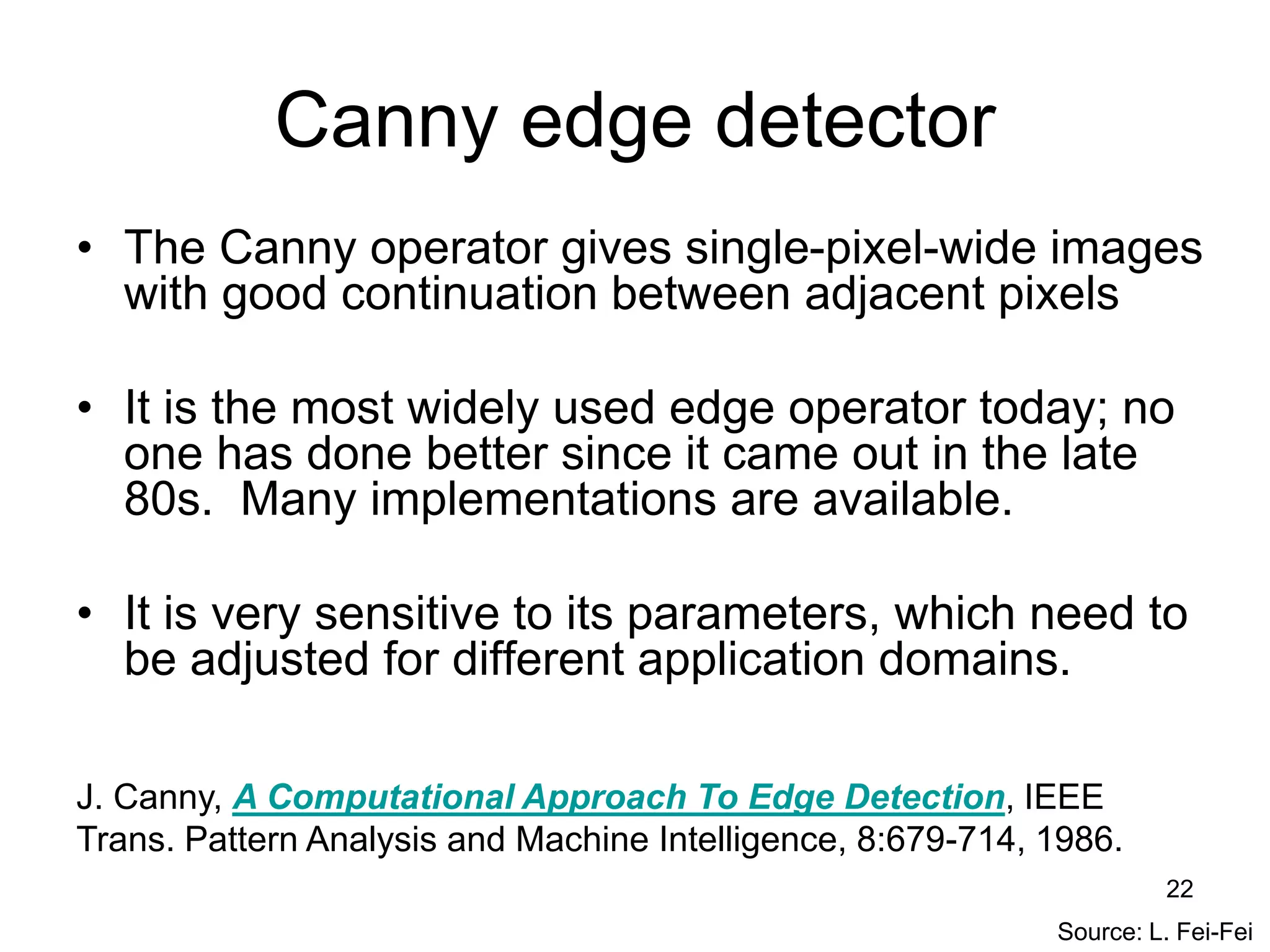
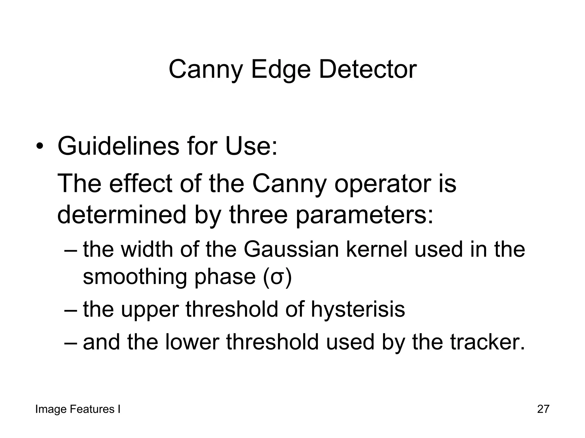
1) The document discusses edge detection and the Hough transform for detecting lines and circles in images. It describes common edge detectors like Sobel, Canny, and LoG and explains how they work. 2) It then introduces the Hough transform as a method to detect lines and circles by having each edge point "vote" for possible lines and circles it could belong to in a parameter space. 3) The Hough transform reduces the complexity from quadratic to linear time compared to examining all pairs of edge points, and is less sensitive to gaps or noise in the edge points.

1. Image Features I
Edges, Lines, Circles
Elsayed Hemayed

2. Overview
• Origin of Edges
• Edge Detectors
– Gradient Operators (Roberts, Prewitt, Sobel).
– Zero Crossing (Canny Edge Detector)
• Detecting Lines and Circles using Hough Transform
Image Features I 2

3. Edge detection
• Convert a 2D image into a set of curves
– Extracts salient features of the scene
– More compact than pixels 3

4. Origin of Edges
• Edges are caused by a variety of factors
depth discontinuity
surface color discontinuity
illumination discontinuity
surface normal discontinuity
Image Features I 4

5. Edge detection
• How can you tell that a pixel is on an
edge?
Image Features I 5

6. Characterizing edges
• An edge is a place of rapid change in the
image intensity function
image
intensity function
(along horizontal scanline) first derivative
edges correspond to
extrema of derivative6

7. Edge detection
1. Detection of short linear edge segments
(edgels)
2. Aggregation of edgels into extended
edges
(maybe parametric description such as
line, circle, …)
Image Features I 7

8. Image gradient
• The gradient of an image:
• The gradient points in the direction of most rapid change in intensity
The gradient direction is given by:
• how does this relate to the direction of the edge?
The edge strength is given by the gradient magnitude
Image Features I 8

9. The gradient direction is given by:
How does this relate to the direction of the edge?
The edge strength is given by the gradient magnitude
Simple image gradient
How would you implement this as a filter?
9
perpendicular
or various
simplifications
0 -1 1

10. Sobel operator
-1 0 1
-2 0 2
-1 0 1
-1 -2 -1
0 0 0
1 2 1
Magnitude:
Orientation:
In practice, it is common to
use:

11. Sobel operator
Original OrientationMagnitude

12. Gradient operators
(a): Roberts’ cross operator (b): 3x3 Prewitt operator
(c): Sobel operator (d) 4x4 Prewitt operator
Image Features I 12

13. Roberts and Prewitt
Image Features I 13

14. Image Features I 14

15. Effects of noise
• Consider a single row or column of the image
– Plotting intensity as a function of position gives a signal
Where is the edge? 15

16. Where is the edge?
Solution: smooth first
Look for peaks in
16

17. Derivative theorem of convolution
• This saves us one operation:
Image Features I 17

18. Laplacian of Gaussian (LoG)
• Consider
Laplacian of Gaussian
operator
Where is the edge? Zero-crossings of bottom graph
18

19. 2D edge detection filters
• is the Laplacian operator:
Laplacian of Gaussian
Gaussian derivative of Gaussian
Image Features I 19

20. Edge detection by subtraction
smoothed (5x5 Gaussian)
original
Original - smoothedImage Features I 20

21. Difference of Gaussians (DoG)
Image Features I 21
DoG LoG

22. Canny edge detector
• The Canny operator gives single-pixel-wide images
with good continuation between adjacent pixels
• It is the most widely used edge operator today; no
one has done better since it came out in the late
80s. Many implementations are available.
• It is very sensitive to its parameters, which need to
be adjusted for different application domains.
J. Canny, A Computational Approach To Edge Detection, IEEE
Trans. Pattern Analysis and Machine Intelligence, 8:679-714, 1986.
Source: L. Fei-Fei
22

23. Steps:
1. Convolve image f with a Gaussian G of
scale σ
2. Filter with Sobel kernel in both horizontal
(gx) and vertical direction (gy)
3. Estimate the local edge gradient for
each pixel.
Canny Edge Detector
Image Features I 23

24. 4. Find the location of the edge using zero
crossing
5. Compute the magnitude of the edge at
that location using
Canny Edge Detector
0*2
2


 fG
n
Image Features I 24

25. 5. Threshold edges with hysteresis to avoid
“streaking problem” (breaking up of the edge
contour caused by operator fluctuating above
and below the threshold).
Thresholding with hysteresis:
1. Two thresholds are set, T1 and T2, T1<T2
2.Responses above T2 are actual edges
3.Responses below T1 are not edges
4.Responses between T1 and T2 are edges if
they are connected to any edges of the strong
response.
Canny Edge Detector
25

26. Guidelines
Sigma Size of Mask
0.5 3x3
1 5x5
2 9x9
3 13x13
4 19x19
15 69 114 69 15
35 155 255 155 35
0 0 0 0 0
-35 -155 -255 -155 -35
-15 -69 -114 -69 -15
15 35 0 -35 -15
69 155 0 155 69
114 255 0 -255 -114
69 155 0 155 69
15 35 0 35 15
x-mask
y-mask
Sigma=1
26

27. • Guidelines for Use:
The effect of the Canny operator is
determined by three parameters:
– the width of the Gaussian kernel used in the
smoothing phase (σ)
– the upper threshold of hysterisis
– and the lower threshold used by the tracker.
Canny Edge Detector
Image Features I 27

28. • Guidelines for Use:
Increasing the width of the Gaussian
kernel reduces the detector's sensitivity to
noise, at the expense of losing some of
the finer detail in the image.
The localization error in the detected
edges also increases slightly as the
Gaussian width is increased.
Canny Edge Detector
Image Features I 28

29. • Usually, the upper tracking threshold can
be set quite high, and the lower threshold
quite low for good results.
• Setting the lower threshold too high will
cause noisy edges to break up.
• Setting the upper threshold too low
increases the number of spurious and
undesirable edge fragments appearing in
the output.
Canny Edge Detector
29

30. Effect of  (Gaussian kernel size)
Canny with Canny withoriginal
The choice of depends on desired behavior
• large detects large scale edges
• small detects fine features 30

31. Canny Edge Detector
Original image St. dev. 1.0
Upper, lower thr.
of 255 and 1
Notice:
Most of the major
edges are detected
 lots of details have
been picked out well
note that this may be
too much detail for
subsequent processing.
Image Features I 31

32. Canny Edge Detector
lowering the upper thr. to 128.
The lower threshold and the
Gaussian st. dev. remains the same
faint edges are detected along
with some short `noisy' fragments
Gaussian used has a st. dev. 2.0.
Same thresholds
Much of the detail on the wall
are no longer detected,
but most of the strong edges remain.
Edges are also smoother and less noisy.
32

33. Image Features I 33

34. fine scale
high
threshold
Image Features I 34

35. coarse
scale,
high
threshold
Image Features I 35

36. coarse
scale
low
threshold
Image Features I 36

37. An edge is not a line...
How can we detect lines ?
Image Features I 37

38. Original Image Edge Image
Finding Curves With Specific
Shape
Target Lines
Image Features I 38

39. Finding lines in an image
• Option 1:
– Search for the line at every possible
position/orientation
– What is the cost of this operation?
• Option 2:
– Use a voting scheme: Hough transform
Image Features I 39

40. Line Grouping Problem
– It is not feasible to check all combinations of features by fitting a model to each
possible subset
– Only some parts of the curve are present
40

41. • Goal:
To find a curve of specific shape (line, circle, … etc) in
an edge image.
• Edges need not be connected
• Key Idea: Edges VOTE for the possible curve
• Computational Complexity:
With n points to find the line connecting each two:
Complexity = n x (n-1)
= n2
Hough transform is computationally attractive!
HoughTransform
Image Features I 41

42. Image and Hough Spaces
cmxy 
),( ii yx
y
x
Equation of Line:
Find:
Consider point:
cmxy 
),( cm
),( ii yx
iiii ymxcorcmxy 
m
),( cm
Image Space
Hough (Parameter) Space
- Every pair of points will form a line
(m, c) and add a vote in the cell
indexed by (m, c)
- The number of votes at (m, c)
Corresponds to the number of points
that lie on the line (m, c). 42
c

43. • Connection between image (x,y) and Hough (m,b)
spaces
– A line in the image corresponds to a point in Hough
space
– To go from image space to Hough space:
• given a set of points (x,y), find all (m,b) such that y = mx + b
x
y
m
b
m0
b0
image space Hough space
Finding lines in an image
43

44. 1. Parameter space is divided into accumulator
cells A, all, initially, set to zero.
2. For every point p(x,y) in image, change m in the
range and calculate c. c=-xm+y
3. A(m, c) = A(m, c) + 1
At the end the value of A(mi, cj) corresponds to the number
of points that lie on the line:
y = - mi x + cj
Algorithm: Hough Transform for line
detection
Image Features I 44

45. • Accuracy of co-linearity is determined by the
size of subdivisions.
• Having m subdivisions, computational
complexity is now
n x m
where m is the number of subdivisions
i.e. linear in n.
Algorithm: Hough Transform for line
detection (cont.)
Image Features I 45

46. Hough Transform Line Detection Example
Original Image
Notice: many non-
belonging edges
Edge ImageOriginal Image Edge Image
Image Features I 46

47. Parameter Space Detected Lines
Hough Transform Line Detection Example
Image Features I 47

48. Hough Transform Line Detection Example
Original Image Original Image with
superimposed Lines
Detected Lines
Example:
Image Features I 48

49. Better Parameterization
(Hough Space Sinusoid)
NOTE:
• Large Accumulator
• More memory and computations
Improvement:
Line equation:
Here
Given points find
 m
 sincos yxR 
max0
0
RR 
 
(Finite Accumulator Array Size)
),( ii yx ),( R
x
Image Space
R
Hough Space
?
y
R is the perpendicular distance from the line to the origin
 is the angle this perpendicular makes with the x axis
Image Features I 49

50. Hough transform algorithm
1. Initialize H[R, ]=0
2. for each edge point I[x,y] in the image
for  = 0 to 180
H[R, ] += 1
3. Find the value(s) of (R, ) where H[R, ] is
maximum
4. The detected line in the image is given by
 sincos yxR 
 sincos yxR 
Image Features I 50

51. Image space
Votes
Horizontal axis is θ,
vertical is R.
Hough Space Sinusoid Example
51Image Features I

52. Note: Axis of R-θ parameter space is rotated 90o !
Hough Transform Line Detection
Example
52

53. Mechanics of the Hough
Transform
• Difficulties
– how big should the cells be? (too big, and we merge
quite different lines; too small, and noise causes lines
to be missed)
• How many lines?
– Count the peaks in the Hough array
– Treat adjacent peaks as a single peak
• Which points belong to each line?
– Search for points close to the line
– Solve again for line and iterate
Demo: http://www/dai.ed.ac.uk/HIPR2/houghdemo.html 53

54. • If looking for circles, instead of lines the
analytic expression is:
• As there are 3 parameters then the
accumulator data structure must be three
dimensional, i.e. the accumulator cell is
A(a,b,r).
Hough Transform for Circle Detection
22)(2)( rbyax 
Image Features I 54

55. Finding Circles by Hough Transform
Equation of Circle:
222
)()( rbyax ii 
If radius is known:
),( baAAccumulator Array
(2D Hough Space)
Image Features I 55

56. • Again the Hough transform is applied to each point
whose edge magnitude exceeds a certain threshold.
• The processing results correspond to points of local
maxima of accumulator cells in the parameter space a,b
of the center point of the circle and the radius r.
• If the length of the radius of the circle searched is known
then we can deal with a 2-dimensional parameter space
(for center point coordinates a,b).
Algorithm: Hough Transform for Circle
Detection
Image Features I 56

57. Demo:Hough Transform
Original Circle
●
●●
● point on circle
circles passing through point
loci of centers of circles passing through point
Intersection of circles
specifies center of original
circle
● point on circle
circles passing through point
57

58. Finding Coins
Original Edges (note noise)
58

59. Hough Space For Coins
Penny Quarters
Image Features I 59

60. Detected Coins
Note that because the quarters
and penny are different sizes, a
different Hough transform (with
separate accumulators) was
used for each circle size.
For Hough Applet see
http://www.markschulze.net/java/hough/
60

61. Hough Transform: Comments
• Works on Disconnected Edges
• Relatively insensitive to occlusion
• Effective for simple shapes (lines, circles,
etc)
• Handling inaccurate edge locations
Image Features I 61