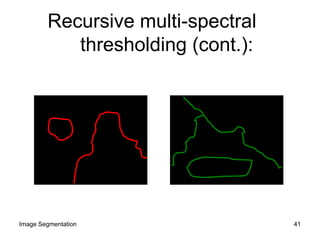
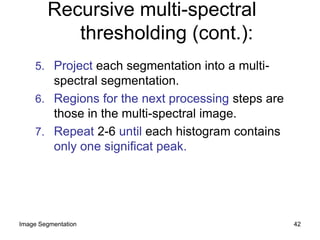
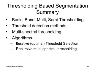
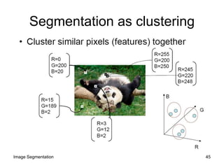
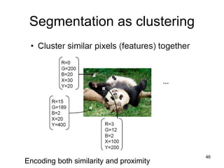
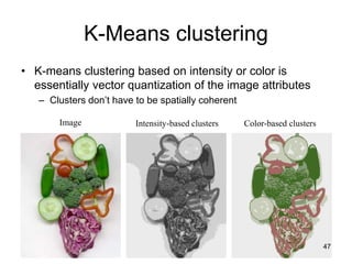
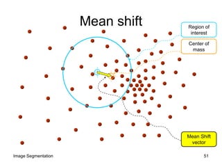
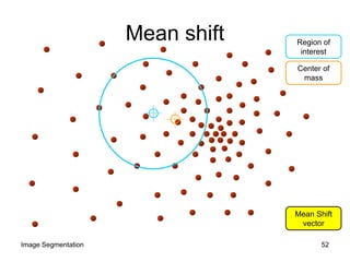
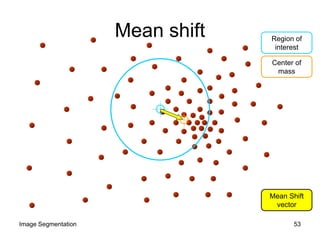
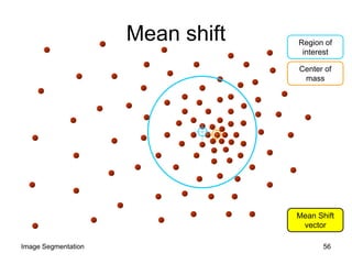
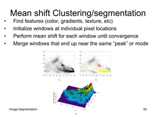
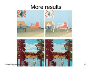
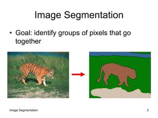
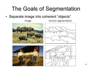
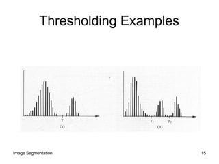
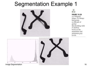
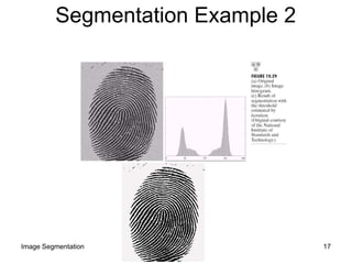
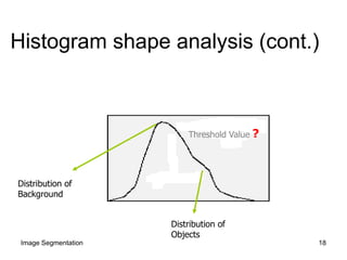
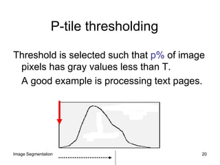
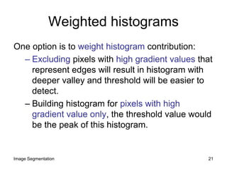
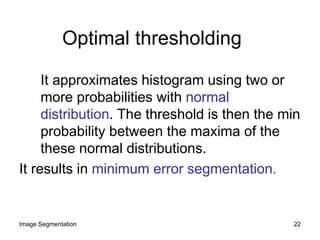
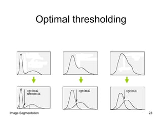
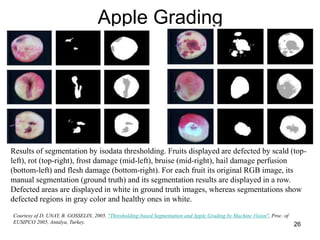
This document discusses various image segmentation techniques including thresholding, clustering, and mean shift segmentation. Thresholding techniques include basic, multi, band, and semi-thresholding. Threshold detection methods analyze the image histogram to select an optimal threshold. Algorithms like iterative threshold selection and recursive multi-spectral thresholding are also presented. Segmentation can also be viewed as a clustering problem, where K-means clustering groups pixels based on intensity or color. Mean shift segmentation treats segmentation as a density estimation problem, using an iterative procedure to locate dense regions in feature space.

1. Image Segmentation
Elsayed Hemayed

2. Overview
• Segmentation
• Thresholding Segmentation Techniques
• Segmentation as clustering
• Mean shift segmentation
2Image Segmentation

3. Image Segmentation
• Goal: identify groups of pixels that go
together
3Image Segmentation

4. The Goals of Segmentation
• Separate image into coherent “objects”
4

5. The Goals of Segmentation
• Separate image into coherent “objects”
• Group together similar‐looking pixels for
efficiency of further processing
5Image Segmentation

6. Segmentation
• Goal: to divide an image into parts that have a
strong correlation with objects or areas of the
real world, mainly objects and background.
• A complete segmentation of an image R is a
set of regions R1, R2, …, Rs
iR
S
i
R
1
  ji RR  ji 
6Image Segmentation

7. Thresholding Segmentation
Technique
• Basic, Band, Multi, Semi-Thresholding
• Threshold detection methods
• Algorithms
– Iterative (optimal) Threshold Selection
– Otsu Segmentation Algorithm
– Recursive multi-spectral thresholding

8. Advantages
• simplest segmentation process since
Many objects or image regions are
characterized by constant reflectivity or
light absorption of their surface.
• computationally inexpensive and fast and
can easily be done in real time
8Image Segmentation

9. Basic Thresholding
• Basic thresholding of an input image f to an output
image g is as follows:
g(i,j) = 1 for f(i,j)
g(i,j) = 0 for f(i,j)
T
T
9Image Segmentation

10. Band Thresholding
• There are several modifications on basic thresholding.
They include:
1. Band thresholding:
g(i,j) = 1 for f(i,j) f(i,j)
g(i,j) = 0 otherwise
• used e.g. in microscopic blood cells
D
10Image Segmentation

11. Multi-Thresholding
2. Multi-thresholding, using limited set of array levels:
g(i,j) = 1 for f(i,j)
g(i,j) = 2 for f(i,j)
g(i,j) = 3 for f(i,j)
.
.
.
g(i,j) = n for f(i,j)
g(i,j) = 0 otherwise
1
D
2
D
3
D
nD
11Image Segmentation

12. Semi-Thresholding
3. Semi-thresholding, masks out background
g(i,j) = f(i,j) for f(i,j)
g(i,j) = 0 for f(i,j)
T
T
12Image Segmentation

13. Threshold Detection techniques
• If some property of an image after segmentation is
known a priori, the task of threshold selection is
simplified, since the threshold is chosen to ensure this
property is satisfied.
• A main detection technique is based on Histogram
shape analysis:
– The chosen threshold is chosen to meet minimum segmentation
error, by selecting it as the gray level that has minimum
histogram value between the two maxima, that represent objects
and background in the image.
13Image Segmentation

14. Histogram shape analysis
Distribution of
Background
Distribution of
Objects
Threshold Value
14Image Segmentation

15. Thresholding Examples
15Image Segmentation

16. Segmentation Example 1
16Image Segmentation

17. Segmentation Example 2
17Image Segmentation

18. Histogram shape analysis (cont.)
Distribution of
Background
Distribution of
Objects
Threshold Value ?
18Image Segmentation

19. Histogram shape analysis
• P-tile thresholding
 Weighted histograms
 Optimal thresholding
19Image Segmentation

20. P-tile thresholding
Threshold is selected such that p% of image
pixels has gray values less than T.
A good example is processing text pages.
20Image Segmentation

21. One option is to weight histogram contribution:
– Excluding pixels with high gradient values that
represent edges will result in histogram with
deeper valley and threshold will be easier to
detect.
– Building histogram for pixels with high
gradient value only, the threshold value would
be the peak of this histogram.
Weighted histograms
21Image Segmentation

22. Optimal thresholding
It approximates histogram using two or
more probabilities with normal
distribution. The threshold is then the min
probability between the maxima of the
these normal distributions.
It results in minimum error segmentation.
22Image Segmentation

23. Optimal thresholding
23Image Segmentation

24. Threshold Detection techniques
Actual Example
24

25. Brain MR Image Segmentation
25

26. Apple Grading
Results of segmentation by isodata thresholding. Fruits displayed are defected by scald (top-
left), rot (top-right), frost damage (mid-left), bruise (mid-right), hail damage perfusion
(bottom-left) and flesh damage (bottom-right). For each fruit its original RGB image, its
manual segmentation (ground truth) and its segmentation results are displayed in a row.
Defected areas are displayed in white in ground truth images, whereas segmentations show
defected regions in gray color and healthy ones in white.
Courtesy of D. UNAY, B. GOSSELIN, 2005, "Thresholding-based Segmentation and Apple Grading by Machine Vision", Proc. of
EUSIPCO 2005, Antalya, Turkey. 26

27. Algorithm: Iterative (optimal)
Threshold Selection
1. As first iteration consider that the 4 corners
contain background pixels only and the
remainder contains object pixels.
2. Calculate and as the average
intensity of background and object pixels.
3. At step t+1 segmentation is performed using
the threshold
t
B t
O
27Image Segmentation

28. Iterative (optimal) Threshold
Selection (cont.)
4. Re-calculate and according to new segmentation
using:
5. Re-calculate
6. Stop if
t
B t
O
)()1( tt
TT 
28Image Segmentation

29. Otsu’s Image Segmentation
Algorithm
• Find the threshold that minimizes the weighted
within-class variance.
• Equivalent to maximizing the between-class
variance.
• Operates directly on the gray level histogram
[e.g. 256 numbers, P(i)]
• It is fast (once the histogram is computed).

30. Otsu: Assumptions
• Histogram (and the image) are bimodal.
• No use of spatial coherence, nor any other notion of
object structure.
• Assumes stationary statistics, but can be modified to
be locally adaptive
• Assumes uniform illumination (implicitly), so the
bimodal brightness behavior arises from object
appearance differences only.

31. The weighted within-class variance is:
w
2
(t)  q1(t)1
2
(t)  q2 (t)2
2
(t)
Where the class probabilities are estimated as:
q1(t)  P(i)
i1
t
 

L
ti
iPtq
1
2 )()(
𝜇1(𝑡) =
1
𝑞1(𝑡)
𝑖=1
𝑡
𝑖𝑃(𝑖) 𝜇2(𝑡) =
1
𝑞2(𝑡)
𝑖=𝑡+1
𝐿
𝑖𝑃(𝑖)
And the class means are given by:
Otsu’s method: Formulation

32. Finally, the individual class variances are:
1
2
(t)  [i  1(t)]2 P(i)
q1(t)i1
t



L
ti tq
iP
tit
1 2
2
2
2
2
)(
)(
)]([)( 
Run through the full range of t values and pick the value that minimizes w
2
(t)
Otsu’s method: Formulation
w
2
(t)  q1(t)1
2
(t)  q2 (t)2
2
(t)

33. Example
Input image Histogram
Global
thresholding
Otsu’s
method

34. Example (in presence of noise)
Input image Histogram Global threshold
Smoothened image Histogram Otsu’s method

35. Image partitioning
Input image Histogram Global threshold
Global Otsu’s Method Image partitioning Local Otsu’s method

36. Thresholding (non-uniform
background)
Input image Global thresholding
using Otsu’s method
Local thresholding
with moving average

37. 1. Initiallize the whole image as a single region.
2. Compute a smoothed histogram for each
spectral band.
3. Find the most significant peak in each
histogram and determine two thresholds on
either sides of the peak.
4. Segment each region in each spectral band into
sub-regions according to these thresholds.
Algorithm: Recursive multi-
spectral thresholding
40Image Segmentation

38. Recursive multi-spectral
thresholding (cont.):
41Image Segmentation

39. 5. Project each segmentation into a multi-
spectral segmentation.
6. Regions for the next processing steps are
those in the multi-spectral image.
7. Repeat 2-6 until each histogram contains
only one significat peak.
Recursive multi-spectral
thresholding (cont.):
42Image Segmentation

40. Demo: Multi-spectral thresholding
43Image Segmentation

41. Thresholding Based Segmentation
Summary
• Basic, Band, Multi, Semi-Thresholding
• Threshold detection methods
• Multi-spectral thresholding
• Algorithms
– Iterative (optimal) Threshold Selection
– Recursive multi-spectral thresholding
44Image Segmentation

42. Segmentation as clustering
45Image Segmentation

43. Segmentation as clustering
Encoding both similarity and proximity
46

44. Image Intensity-based clusters Color-based clusters
K-Means clustering
• K-means clustering based on intensity or color is
essentially vector quantization of the image attributes
– Clusters don’t have to be spatially coherent
47

45. K-Means pros and cons
• Pros
– Simple and fast
– Converges to a local
minimum of the error function
• Cons
– Need to pick K
– Sensitive to initialization
– Sensitive to outliers
– Only finds “spherical”
clusters
48Image Segmentation

46. http://www.caip.rutgers.edu/~comanici/MSPAMI/msPamiResults.html
Mean shift segmentation
• An advanced and versatile technique for clustering-based
segmentation
D. Comaniciu and P. Meer, Mean Shift: A Robust Approach toward Feature
Space Analysis, PAMI 2002.
49

47. • The mean shift algorithm seeks a mode or local
maximum of density of a given distribution
– Choose a search window (width and location)
– Compute the mean of the data in the search window
– Center the search window at the new mean location
– Repeat until convergence
Mean shift algorithm
50Image Segmentation

48. Region of
interest
Center of
mass
Mean Shift
vector
Mean shift
51Image Segmentation

49. Region of
interest
Center of
mass
Mean Shift
vector
Mean shift
52Image Segmentation

50. Region of
interest
Center of
mass
Mean Shift
vector
Mean shift
53Image Segmentation

51. Region of
interest
Center of
mass
Mean Shift
vector
Mean shift
54Image Segmentation

52. Region of
interest
Center of
mass
Mean Shift
vector
Mean shift
55Image Segmentation

53. Region of
interest
Center of
mass
Mean Shift
vector
Mean shift
56Image Segmentation

54. Region of
interest
Center of
mass
Mean shift
57Image Segmentation

55. • Cluster: all data points in the attraction basin of a mode
• Attraction basin: the region for which all trajectories lead
to the same mode
Mean shift clustering
58Image Segmentation

56. • Find features (color, gradients, texture, etc)
• Initialize windows at individual pixel locations
• Perform mean shift for each window until convergence
• Merge windows that end up near the same “peak” or mode
Mean shift Clustering/segmentation
59Image Segmentation

57. http://www.caip.rutgers.edu/~comanici/MSPAMI/msPamiResults.html
Mean shift segmentation results
60

58. More results
61Image Segmentation

59. More results
62Image Segmentation

60. Mean shift pros and cons
• Pros
– Does not assume spherical clusters
– Just a single parameter (window size)
– Finds variable number of modes
– Robust to outliers
• Cons
– Output depends on window size
– Computationally expensive
– Does not scale well with dimension of feature space
63Image Segmentation