Download as PDF, PPTX

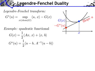
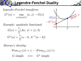
![Convex Optimization
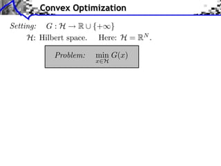
Setting: G : H
R ⇤ {+⇥}
H: Hilbert space. Here: H = RN .
Problem:
Class of functions:
Convex: G(tx + (1
min G(x)
x H
y
x
t)y)
tG(x) + (1
t)G(y)
t
[0, 1]](https://image.slidesharecdn.com/2013-12-16-jga-3-131217031308-phpapp02/85/Low-Complexity-Regularization-of-Inverse-Problems-Course-3-Proximal-Splitting-Methods-4-320.jpg)
![Convex Optimization
Setting: G : H
R ⇤ {+⇥}
H: Hilbert space. Here: H = RN .
Problem:
Class of functions:
Convex: G(tx + (1
min G(x)
x H
y
x
t)y)
Lower semi-continuous:
tG(x) + (1
t)G(y)
lim inf G(x)
G(x0 )
x
x0
Proper: {x ⇥ H G(x) ⇤= + } = ⌅
⇤
t
[0, 1]](https://image.slidesharecdn.com/2013-12-16-jga-3-131217031308-phpapp02/85/Low-Complexity-Regularization-of-Inverse-Problems-Course-3-Proximal-Splitting-Methods-5-320.jpg)
![Convex Optimization
Setting: G : H
R ⇤ {+⇥}
H: Hilbert space. Here: H = RN .
min G(x)
Problem:
Class of functions:
Convex: G(tx + (1
x H
t)y)
Lower semi-continuous:
tG(x) + (1
t)G(y)
lim inf G(x)
G(x0 )
x
x0
Proper: {x ⇥ H G(x) ⇤= + } = ⌅
⇤
Indicator:
y
x
C (x)
=
(C closed and convex)
0 if x ⇥ C,
+
otherwise.
t
[0, 1]](https://image.slidesharecdn.com/2013-12-16-jga-3-131217031308-phpapp02/85/Low-Complexity-Regularization-of-Inverse-Problems-Course-3-Proximal-Splitting-Methods-6-320.jpg)
![Sub-differential
Sub-di erential:
G(x) = {u ⇥ H ⇤ z, G(z)
G(x) + ⌅u, z
x⇧}
G(x) = |x|
G(0) = [ 1, 1]](https://image.slidesharecdn.com/2013-12-16-jga-3-131217031308-phpapp02/85/Low-Complexity-Regularization-of-Inverse-Problems-Course-3-Proximal-Splitting-Methods-12-320.jpg)
![Sub-differential
Sub-di erential:
G(x) = {u ⇥ H ⇤ z, G(z)
Smooth functions:
G(x) + ⌅u, z
x⇧}
G(x) = |x|
If F is C 1 , F (x) = { F (x)}
G(0) = [ 1, 1]](https://image.slidesharecdn.com/2013-12-16-jga-3-131217031308-phpapp02/85/Low-Complexity-Regularization-of-Inverse-Problems-Course-3-Proximal-Splitting-Methods-13-320.jpg)
![Sub-differential
Sub-di erential:
G(x) = {u ⇥ H ⇤ z, G(z)
G(x) + ⌅u, z
x⇧}
G(x) = |x|
Smooth functions:
If F is C 1 , F (x) = { F (x)}
G(0) = [ 1, 1]
First-order conditions:
x
argmin G(x)
x H
0
G(x )](https://image.slidesharecdn.com/2013-12-16-jga-3-131217031308-phpapp02/85/Low-Complexity-Regularization-of-Inverse-Problems-Course-3-Proximal-Splitting-Methods-14-320.jpg)
![Sub-differential
Sub-di erential:
G(x) = {u ⇥ H ⇤ z, G(z)
G(x) + ⌅u, z
x⇧}
G(x) = |x|
Smooth functions:
If F is C 1 , F (x) = { F (x)}
G(0) = [ 1, 1]
First-order conditions:
x
argmin G(x)
0
x H
Monotone operator:
(u, v)
U (x)
G(x )
U (x)
x
U (x) = G(x)
U (y),
y
x, v
u
0](https://image.slidesharecdn.com/2013-12-16-jga-3-131217031308-phpapp02/85/Low-Complexity-Regularization-of-Inverse-Problems-Course-3-Proximal-Splitting-Methods-15-320.jpg)
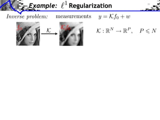
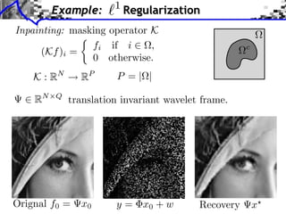
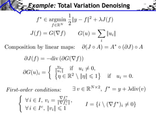
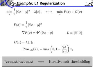
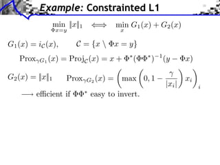
![Example:
1
Regularization
1
x ⇥ argmin G(x) = ||y
2
x RQ
⇥G(x) =
|| · ||1 (x)i =
( x
y) + ⇥|| · ||1 (x)
x||2 + ||x||1
sign(xi ) if xi ⇥= 0,
[ 1, 1] if xi = 0.](https://image.slidesharecdn.com/2013-12-16-jga-3-131217031308-phpapp02/85/Low-Complexity-Regularization-of-Inverse-Problems-Course-3-Proximal-Splitting-Methods-16-320.jpg)
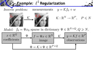
![Example:
1
Regularization
1
x ⇥ argmin G(x) = ||y
2
x RQ
⇥G(x) =
|| · ||1 (x)i =
( x
x||2 + ||x||1
y) + ⇥|| · ||1 (x)
sign(xi ) if xi ⇥= 0,
[ 1, 1] if xi = 0.
Support of the solution:
I = {i ⇥ {0, . . . , N 1} xi ⇤= 0}
xi
i](https://image.slidesharecdn.com/2013-12-16-jga-3-131217031308-phpapp02/85/Low-Complexity-Regularization-of-Inverse-Problems-Course-3-Proximal-Splitting-Methods-17-320.jpg)
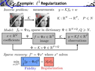
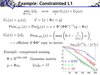
![Example:
1
Regularization
1
x ⇥ argmin G(x) = ||y
2
x RQ
⇥G(x) =
|| · ||1 (x)i =
( x
x||2 + ||x||1
y) + ⇥|| · ||1 (x)
sign(xi ) if xi ⇥= 0,
[ 1, 1] if xi = 0.
xi
i
Support of the solution:
I = {i ⇥ {0, . . . , N 1} xi ⇤= 0}
First-order conditions:
s
RN ,
( x
i,
y) + s = 0
sI = sign(xI ),
||sI c ||
1.
y
x
i](https://image.slidesharecdn.com/2013-12-16-jga-3-131217031308-phpapp02/85/Low-Complexity-Regularization-of-Inverse-Problems-Course-3-Proximal-Splitting-Methods-18-320.jpg)
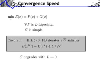
![Gradient and Proximal Descents
x( +1) = x( )
G(x( ) )
Gradient descent:
G is C 1 and G is L-Lipschitz
Theorem:
If 0 <
< 2/L, x(
)
[explicit]
x a solution.](https://image.slidesharecdn.com/2013-12-16-jga-3-131217031308-phpapp02/85/Low-Complexity-Regularization-of-Inverse-Problems-Course-3-Proximal-Splitting-Methods-32-320.jpg)
![Gradient and Proximal Descents
x( +1) = x( )
G(x( ) )
Gradient descent:
G is C 1 and G is L-Lipschitz
Theorem:
< 2/L, x(
If 0 <
Sub-gradient descent: x(
Theorem:
If
+1)
= x(
1/⇥, x(
Problem: slow.
)
)
)
[explicit]
x a solution.
v( ) ,
v(
)
x a solution.
G(x( ) )](https://image.slidesharecdn.com/2013-12-16-jga-3-131217031308-phpapp02/85/Low-Complexity-Regularization-of-Inverse-Problems-Course-3-Proximal-Splitting-Methods-33-320.jpg)
![Gradient and Proximal Descents
x( +1) = x( )
G(x( ) )
Gradient descent:
G is C 1 and G is L-Lipschitz
Theorem:
< 2/L, x(
If 0 <
Sub-gradient descent: x(
Theorem:
+1)
= x(
1/⇥, x(
If
)
)
[explicit]
x a solution.
v( ) ,
v(
)
G(x( ) )
x a solution.
)
Problem: slow.
Proximal-point algorithm: x(⇥+1) = Prox
Theorem:
c > 0, x(
If
Prox
G
)
(x(⇥) ) [implicit]
G
x a solution.
hard to compute.](https://image.slidesharecdn.com/2013-12-16-jga-3-131217031308-phpapp02/85/Low-Complexity-Regularization-of-Inverse-Problems-Course-3-Proximal-Splitting-Methods-34-320.jpg)
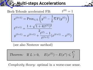
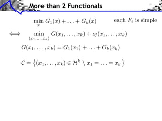
![Block Regularization
1
2
block sparsity: G(x) =
b B
iments
2
+
(2)
` 1 `2
4
k=1
N: 256
x
x2
m
m b
Towards More Complex Penalization
Bk
1,2
⇥ x⇥⇥1 =
i ⇥xi ⇥
b
Image f =
||x[b] ||2 =
||x[b] ||,
B
x Coe cients x.
b B
i
xi2
b
b B1
b B2
+
i b xi
i b xi](https://image.slidesharecdn.com/2013-12-16-jga-3-131217031308-phpapp02/85/Low-Complexity-Regularization-of-Inverse-Problems-Course-3-Proximal-Splitting-Methods-69-320.jpg)
![Block Regularization
1
2
block sparsity: G(x) =
b B
||x[b] ||,
||x[b] ||2 =
x2
m
m b
... B
Non-overlapping decomposition: B = B
iments Towards More Complex Penalization
Towards More Complex Penalization
Towards More Complex Penalization
2
1
n
(2)
G(x) =4 x iBk
(x)
+ ` ` k=1 G 1,2
1
2
N: 256
Gi (x) =
b Bi
i=1
⇥=
⇥ x⇥x⇥x⇥⇥1 =i ⇥x⇥x⇥xi ⇥
⇥ ⇥1 ⇥1 = i i ⇥i i ⇥
b
Image f =
||x[b] ||,
bb B B i
Bb
xii2bi2xi2
bbx
i
B
x Coe cients x.
n
Blocks B1
22
b b 1b1 B1 i b xiixb xi
BB
i b i
++ +
b b 2b2 B2 i
BB
B1
xi2 b2xi
b b xi
i
B2](https://image.slidesharecdn.com/2013-12-16-jga-3-131217031308-phpapp02/85/Low-Complexity-Regularization-of-Inverse-Problems-Course-3-Proximal-Splitting-Methods-70-320.jpg)
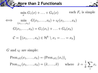
![Block Regularization
1
2
block sparsity: G(x) =
b B
||x[b] ||,
||x[b] ||2 =
x2
m
m b
... B
Non-overlapping decomposition: B = B
iments Towards More Complex Penalization
Towards More Complex Penalization
Towards More Complex Penalization
2
1
n
(2)
G(x) =4 x iBk
(x)
+ ` ` k=1 G 1,2
1
2
Gi (x) =
b Bi
i=1
||x[b] ||,
Each Gi is simple:
⇥ ⇥1 = i ⇥i i
⇥ x⇥x⇥x⇥⇥1 =i ⇥xG ⇥xi ⇥ m = b B B i b xii2bi2xi2
=
Bb
⇤ m ⇥ b ⇥ Bi , ⇥ ⇥1Prox i ⇥xi ⇥(x) b max i0, 1
bx
N: 256
b
Image f =
B
x Coe cients x.
n
Blocks B1
22
b b 1b1 B1 i b xiixb xi
BB
i b i
||x[b]b||B
b B b
++m
x +
2 2 B2
B1
i
xi2 b2xi
b b xi
i
B2](https://image.slidesharecdn.com/2013-12-16-jga-3-131217031308-phpapp02/85/Low-Complexity-Regularization-of-Inverse-Problems-Course-3-Proximal-Splitting-Methods-71-320.jpg)
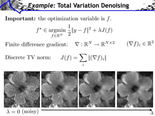
![Example: TV Denoising
1
min ||f
f RN 2
y||2 + ||⇥f ||1
||u||1 =
Dual solution u
i
||ui ||
min ||y + div(u)||2
||u||
||u||
= max ||ui ||
i
Primal solution f = y + div(u )
[Chambolle 2004]](https://image.slidesharecdn.com/2013-12-16-jga-3-131217031308-phpapp02/85/Low-Complexity-Regularization-of-Inverse-Problems-Course-3-Proximal-Splitting-Methods-87-320.jpg)
![Example: TV Denoising
1
min ||f
f RN 2
min ||y + div(u)||2
y||2 + ||⇥f ||1
||u||1 =
Dual solution u
i
||u||
||u||
||ui ||
+1)
= Proj||·||
i
Primal solution f = y + div(u )
FB (aka projected gradient descent):
u(
= max ||ui ||
u( ) +
[Chambolle 2004]
(y + div(u( ) ))
ui
v = Proj||·||
(u)
vi =
max(||ui ||/ , 1)
2
1
<
=
Convergence if
||div ⇥||
4](https://image.slidesharecdn.com/2013-12-16-jga-3-131217031308-phpapp02/85/Low-Complexity-Regularization-of-Inverse-Problems-Course-3-Proximal-Splitting-Methods-88-320.jpg)
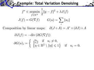
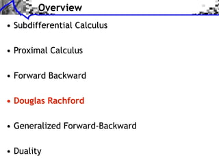
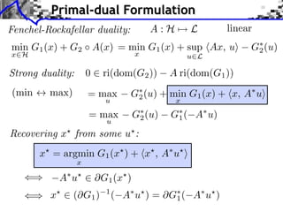
![Primal-Dual Algorithm
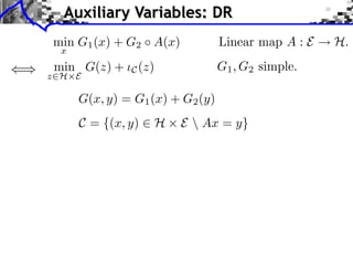
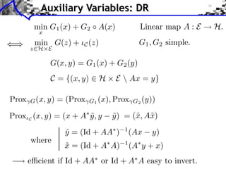
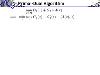
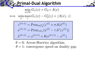
min G1 (x) + G2 A(x)
x H
G⇤ (z) + hA(x), zi
2
() min max G1 (x)
x
z
z (`+1) = Prox
G⇤
2
x(⇥+1) = Prox
(x(⇥)
G1
x(
˜
+ (x(
+1)
= x(
+1)
(z (`) + A(˜(`) )
x
A (z (⇥) ))
+1)
x( ) )
= 0: Arrow-Hurwicz algorithm.
= 1: convergence speed on duality gap.
Theorem: [Chambolle-Pock 2011]
If 0
x(
)
1 and ⇥⇤ ||A||2 < 1 then
x minimizer of G1 + G2 A.](https://image.slidesharecdn.com/2013-12-16-jga-3-131217031308-phpapp02/85/Low-Complexity-Regularization-of-Inverse-Problems-Course-3-Proximal-Splitting-Methods-91-320.jpg)
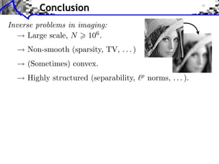
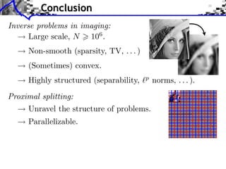

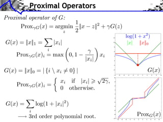
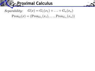
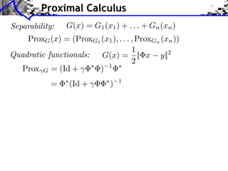
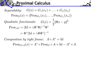
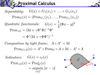
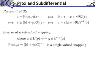
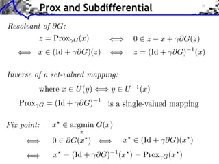
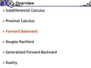
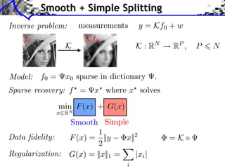
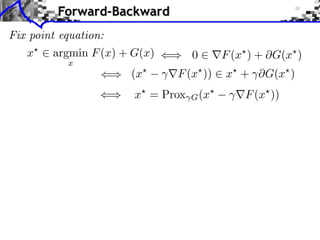
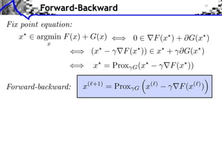
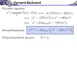
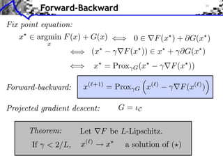
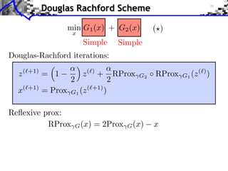
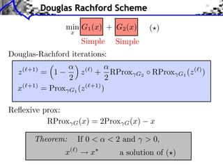
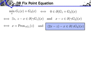
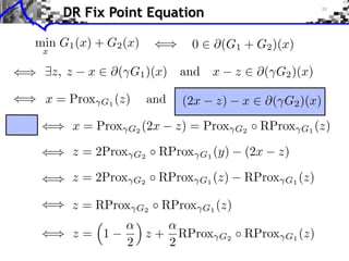
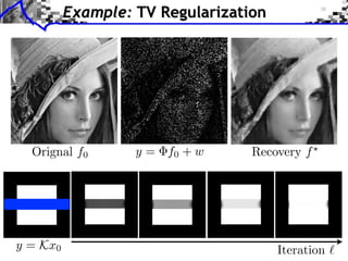
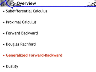
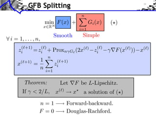
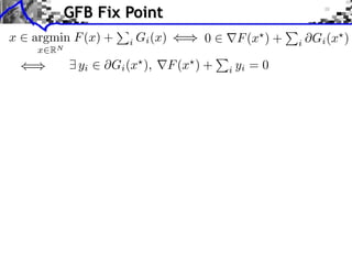
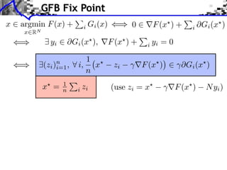
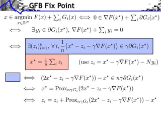
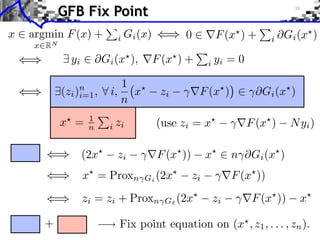
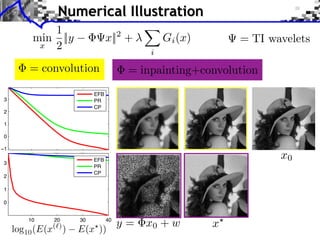
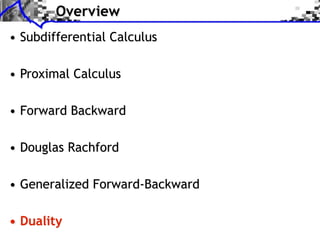
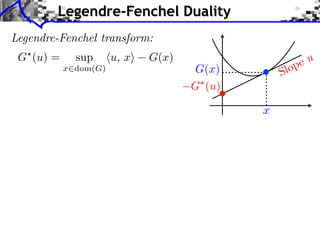
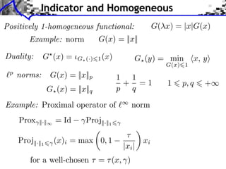
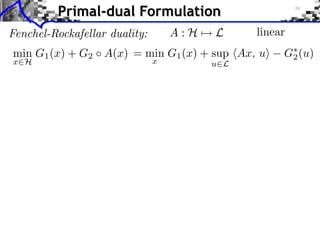
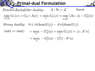
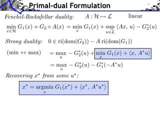
The document discusses proximal splitting methods for solving optimization problems involving the minimization of a sum of functions. It first introduces subdifferential calculus and proximal operators. It then describes several proximal splitting algorithms, including forward-backward splitting, Douglas-Rachford splitting, primal-dual splitting, and generalized forward-backward splitting. These algorithms allow solving composite optimization problems by exploiting the separable structure and properties like smoothness or proximity of the individual terms. The document provides examples of applying such methods to inverse problems like sparse recovery.