Download to read offline

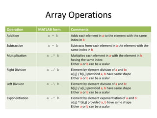
![Operations on Vectors and Matrices
v=[3 7 2 1]
for i = 1:length(v)
v(i) =v(i) * 3;
end
v= [3 7 2 1];
>> v=v*3
9 27 6 3
mat = [4:6; 3:-1:1]
mat =
4 5 6
3 2 1
>> mat * 2
ans =
8 10 12
6 4 2](https://image.slidesharecdn.com/csci101lect09vectorizedcode-200319121959/85/Csci101-lect09-vectorized_code-3-320.jpg)
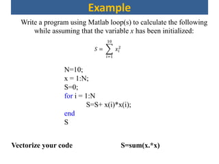
![Element Operations
Both arrays must have the same number of rows and columns
A + B = [1 2 3] + [3 4 5] = [4 6 8]
Element and Algebraic operations are the same
A .* B = [1 2 3] .* [3 4 5] = [3 8 15]
A .^ B = [4 9 6] .^ [2 2 2] = [16 81 36]
A ./ B =[4 9 6] ./ [2 3 2] = [2 3 3]](https://image.slidesharecdn.com/csci101lect09vectorizedcode-200319121959/85/Csci101-lect09-vectorized_code-5-320.jpg)
![Operations Rules Examples
v=[3 7 2 1];
>> v ^ 2
??? Error using ==> mpower
Inputs must be a scalar and a square matrix.
To compute elementwise POWER, use POWER (.^)
instead.
>> v .^ 2
ans =
9 49 4 1](https://image.slidesharecdn.com/csci101lect09vectorizedcode-200319121959/85/Csci101-lect09-vectorized_code-7-320.jpg)
![Operations Rules Examples
v1 = 2:5;
v1 = [2 3 4 5]
v2 = [33 11 5 1];
>> v1 * v2 %Error why
>> v1*v2’ % what is the output
>> v1 .* v2 % v1 and v2 must have same size](https://image.slidesharecdn.com/csci101lect09vectorizedcode-200319121959/85/Csci101-lect09-vectorized_code-8-320.jpg)
![Vectors and Matrices as Function
Arguments
• Many functions accept scalars as input
• Some functions work on arrays
• Most scalar functions accept arrays as well
– The function is performed on each element in the array
individually
• Try x = pi/2; y = sin(x) in MATLAB
• Now try
x = [0 pi/2 pi 3*pi/2 2*pi];
y = sin(x)](https://image.slidesharecdn.com/csci101lect09vectorizedcode-200319121959/85/Csci101-lect09-vectorized_code-9-320.jpg)
![Functions Examples
v1=[1 3 2 7 4 -2]
v2=[5 3 4 1 2 -2]
[mx mxi]=max(v1) 7 4
v=v1-v2 -4 0 -2 6 2 0
v=sign(v1-v2) -1 0 -1 1 1 0
x=sum(v1) 15
v=find(v1>3) 4 5](https://image.slidesharecdn.com/csci101lect09vectorizedcode-200319121959/85/Csci101-lect09-vectorized_code-10-320.jpg)
![Logical Vectors
v1=[1 3 2 7 4 -2]
v2=[5 3 -4 -1 2 -2]
v=v1>0 1 1 1 1 1 0
v=v2>0 1 1 0 0 1 0
a=v2(v2>0) 5 3 2
x=sum(v2>0) 3
v=true(1,5) 1 1 1 1 1
v=false(1,5) 0 0 0 0 0
x=all(v1>0) 1 (are all ones?)
y=any(v1>0) 0 (any one?)](https://image.slidesharecdn.com/csci101lect09vectorizedcode-200319121959/85/Csci101-lect09-vectorized_code-11-320.jpg)
![Example
?)0:),1((ofvaluetheisWhat
5310
2412
3142
0311
aBaLet
B = [0 0 0 1]](https://image.slidesharecdn.com/csci101lect09vectorizedcode-200319121959/85/Csci101-lect09-vectorized_code-12-320.jpg)
![Example
?)2:1],34([ofvaluetheisWhat
5310
2412
3142
0311
aDaLet
12
10
D](https://image.slidesharecdn.com/csci101lect09vectorizedcode-200319121959/85/Csci101-lect09-vectorized_code-13-320.jpg)
![Getting Maximum and Minimum Value
v=[1 3 2 7 4 2]
maxv=0;
for =1:length(v)
if v(i)>maxv
maxv=v(i);
maxi=i;
end
end
% Repeat for the minimum
i v(i) maxv maxi
1 1 01 ?1
2 3 13 12
3 2 3 2
4 7 37 24
5 4 7 4
6 2 7 4
Vectorize your code: [maxv maxi]=max(v)
Example](https://image.slidesharecdn.com/csci101lect09vectorizedcode-200319121959/85/Csci101-lect09-vectorized_code-15-320.jpg)
![Counting Elements
v=[1 3 2 -7 4 -2]
c=0;
for =1:length(v)
if v(i)>0
c=c+1;
end
end
% Repeat for the negative
i v(i) c
1 1 01
2 3 12
3 2 23
4 -7 3
5 4 34
6 -2 4
Vectorize your code c = sum(v>0)
Example](https://image.slidesharecdn.com/csci101lect09vectorizedcode-200319121959/85/Csci101-lect09-vectorized_code-16-320.jpg)
![Comparing Elements
v1=[1 3 2 7 4 -2]
v2=[5 3 4 1 2 -2]
for i=1:length(v1)
if v1(i)>v2(i)
v(i)=1;
else
v(i)=0;
end
end
i v1(i) v2(i) v(i)
1 1 5 0
2 3 3 0
3 2 4 0
4 7 1 1
5 4 2 1
6 -2 -2 0
Vectorize your code: v= v1>v2
Example](https://image.slidesharecdn.com/csci101lect09vectorizedcode-200319121959/85/Csci101-lect09-vectorized_code-17-320.jpg)
![Vertical Motion
% Vertical motion under gravity
g = 9.81; % acceleration due to gravity
u = 60; % initial velocity in metres/sec
t = 0 : 0.1 : 12.3; % time in seconds
s = u * t – g / 2 * t .ˆ 2; % vertical displacement in metres
plot(t, s), title( ’Vertical motion under gravity’ )
xlabel( ’time’ ), ylabel( ’vertical displacement’ )
grid
disp( [t’ s’] ) % display a table
Example](https://image.slidesharecdn.com/csci101lect09vectorizedcode-200319121959/85/Csci101-lect09-vectorized_code-18-320.jpg)

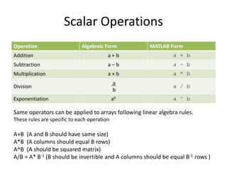
This document discusses vectorized code in MATLAB. It covers operations on vectors and matrices such as addition, subtraction, and multiplication. It discusses using vectors and matrices as function arguments and performing element-wise operations. It also covers logical vectors and examples of vectorizing code using loops to perform operations such as finding maximum/minimum values, counting elements, and comparing elements in less than 3 sentences.