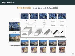
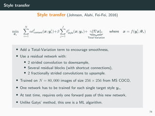
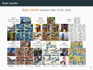
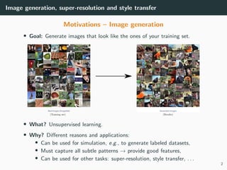
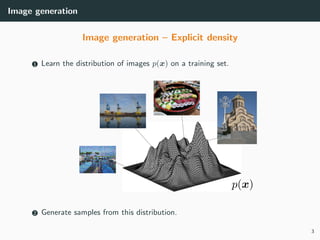
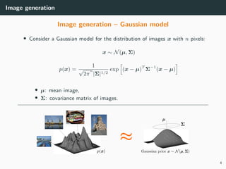
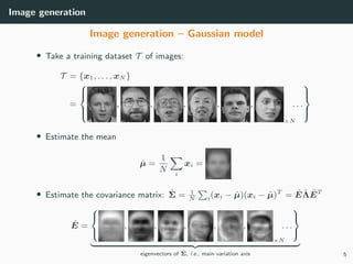
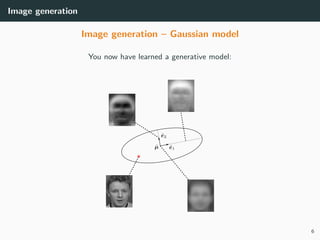
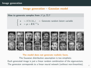
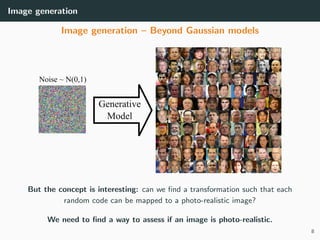
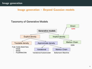
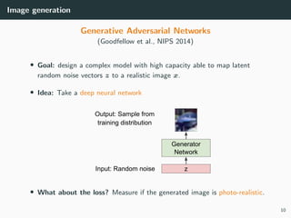
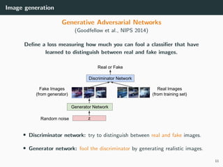
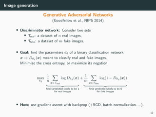
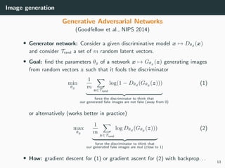
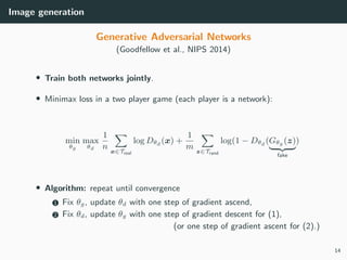
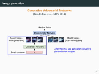
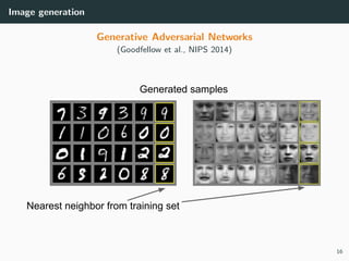
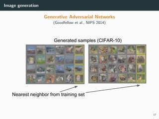
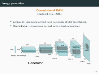
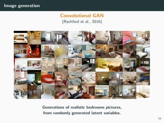
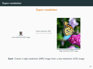
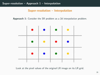
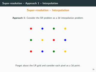
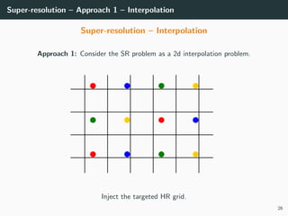
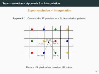
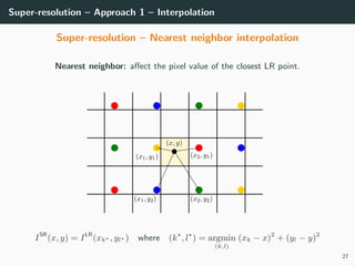
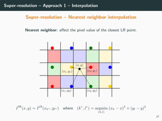
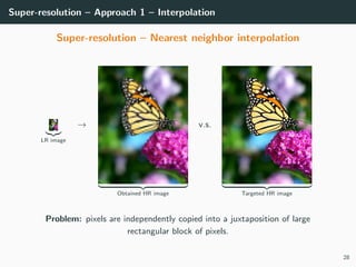
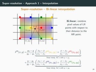
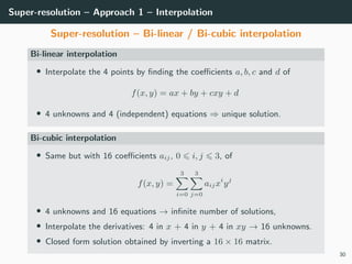
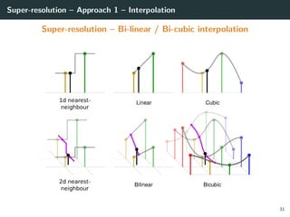
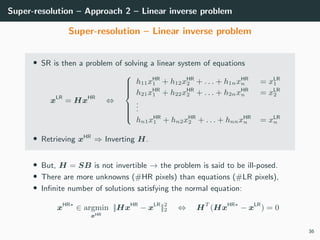
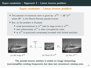
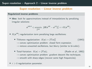
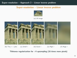
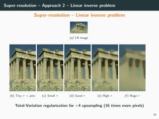
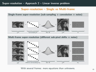
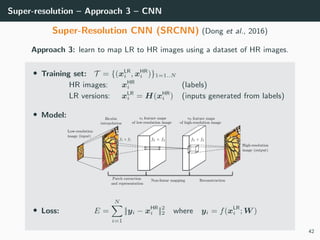
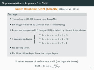
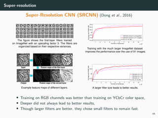
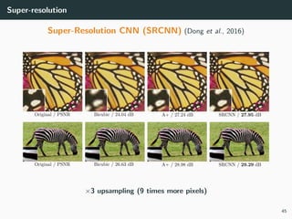
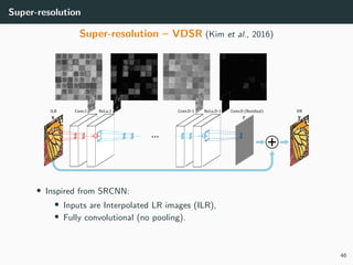
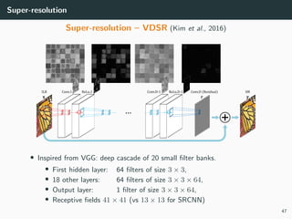
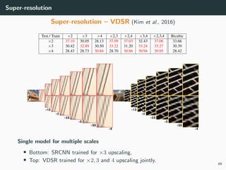
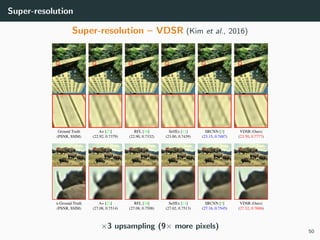
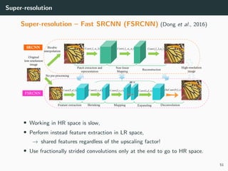
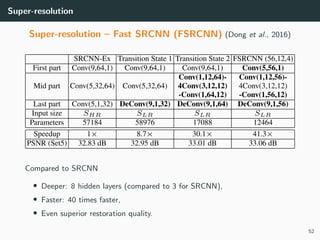
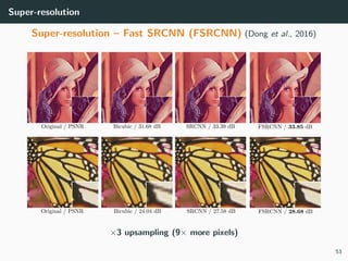
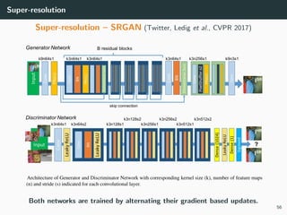
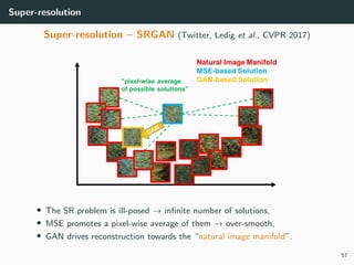
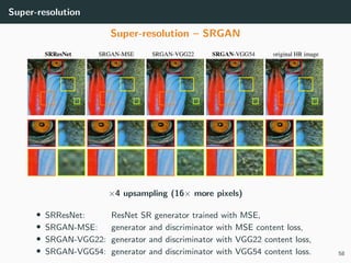
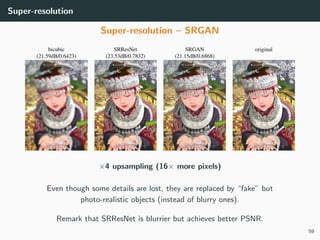
The document discusses various techniques in image generation, super-resolution, and style transfer, focusing particularly on Generative Adversarial Networks (GANs) and their applications. It outlines the goals of generating realistic images from training datasets while detailing different models and approaches to achieve super-resolution. The document elaborates on challenges, including ill-posed problems in reconstruction and the necessity for advanced optimizations to produce high-quality images.

1. ECE 285
Machine Learning for Image Processing
Chapter VI – Generation, super-resolution and style transfer
Charles Deledalle
March 11, 2019
1

2. Image generation

3. Image generation, super-resolution and style transfer
Motivations – Image generation
• Goal: Generate images that look like the ones of your training set.
• What? Unsupervised learning.
• Why? Different reasons and applications:
• Can be used for simulation, e.g., to generate labeled datasets,
• Must capture all subtle patterns → provide good features,
• Can be used for other tasks: super-resolution, style transfer, . . .
2

4. Image generation
Image generation – Explicit density
1 Learn the distribution of images p(x) on a training set.
2 Generate samples from this distribution.
3

5. Image generation
Image generation – Gaussian model
• Consider a Gaussian model for the distribution of images x with n pixels:
x ∼ N(µ, Σ)
p(x) =
1
√
2π
n
|Σ|1/2
exp (x − µ)T
Σ−1
(x − µ)
• µ: mean image,
• Σ: covariance matrix of images.
4

6. Image generation
Image generation – Gaussian model
• Take a training dataset T of images:
T = {x1, . . . , xN }
=



, , , , ,
×N
, . . .



• Estimate the mean
ˆµ =
1
N i
xi =
• Estimate the covariance matrix: ˆΣ = 1
N i(xi − ˆµ)(xi − ˆµ)T
= ˆE ˆΛ ˆET
ˆE =



, , , , ,
×N
, . . .



eigenvectors of ˆΣ, i.e., main variation axis 5

7. Image generation
Image generation – Gaussian model
You now have learned a generative model:
6

8. Image generation
Image generation – Gaussian model
How to generate samples from N(ˆµ, ˆΣ)?
z ∼ N(0, Idn) ← Generate random latent variable
x = ˆµ + ˆE ˆΛ1/2
z
The model does not generate realistic faces.
The Gaussian distribution assumption is too simplistic.
Each generated image is just a linear random combination of the eigenvectors.
The generator corresponds to a linear neural network (without non-linearities). 7

9. Image generation
Image generation – Beyond Gaussian models
But the concept is interesting: can we find a transformation such that each
random code can be mapped to a photo-realistic image?
We need to find a way to assess if an image is photo-realistic.
8

10. Image generation
Image generation – Beyond Gaussian models
9

11. Image generation
Generative Adversarial Networks
(Goodfellow et al., NIPS 2014)
• Goal: design a complex model with high capacity able to map latent
random noise vectors z to a realistic image x.
• Idea: Take a deep neural network
• What about the loss? Measure if the generated image is photo-realistic.
10

12. Image generation
Generative Adversarial Networks
(Goodfellow et al., NIPS 2014)
Define a loss measuring how much you can fool a classifier that have
learned to distinguish between real and fake images.
• Discriminator network: try to distinguish between real and fake images.
• Generator network: fool the discriminator by generating realistic images.
11

13. Image generation
Generative Adversarial Networks
(Goodfellow et al., NIPS 2014)
• Discriminator network: Consider two sets
• Treal: a dataset of n real images,
• Tfake: a dataset of m fake images.
• Goal: find the parameters θd of a binary classification network
x → Dθd (x) meant to classify real and fake images.
Minimize the cross entropy, or maximize its negation
max
θd
1
n x∈Treal
log Dθd (x)
force predicted labels to be 1
for real images
+
1
m x∈Tfake
log(1 − Dθd (x))
force predicted labels to be 0
for fake images
• How: use gradient ascent with backprop (+SGD, batch-normalization. . . ).
12

14. Image generation
Generative Adversarial Networks
(Goodfellow et al., NIPS 2014)
• Generator network: Consider a given discriminative model x → Dθd (x)
and consider Trand a set of m random latent vectors.
• Goal: find the parameters θg of a network x → Gθg (z) generating images
from random vectors z such that it fools the discriminator
min
θg
1
m z∈Trand
log(1 − Dθd (Gθg (z)))
force the discriminator to think that
our generated fake images are not fake (away from 0)
(1)
or alternatively (works better in practice)
max
θg
1
m z∈Trand
log Dθd (Gθg (z)))
force the discriminator to think that
our generated fake images are real (close to 1)
(2)
• How: gradient descent for (1) or gradient ascent for (2) with backprop. . .
13

15. Image generation
Generative Adversarial Networks
(Goodfellow et al., NIPS 2014)
• Train both networks jointly.
• Minimax loss in a two player game (each player is a network):
min
θg
max
θd
1
n x∈Treal
log Dθd (x) +
1
m z∈Trand
log(1 − Dθd (Gθg (z)
fake
)
• Algorithm: repeat until convergence
1 Fix θg, update θd with one step of gradient ascend,
2 Fix θd, update θg with one step of gradient descent for (1),
(or one step of gradient ascent for (2).)
14

16. Image generation
Generative Adversarial Networks
(Goodfellow et al., NIPS 2014)
15

17. Image generation
Generative Adversarial Networks
(Goodfellow et al., NIPS 2014)
16

18. Image generation
Generative Adversarial Networks
(Goodfellow et al., NIPS 2014)
17

19. Image generation
Convolutional GAN
(Rachford et al., 2016)
• Generator: upsampling network with fractionally strided convolutions,
• Discriminator: convolutional network with strided convolutions.
18

20. Image generation
Convolutional GAN
(Rachford et al., 2016)
Generations of realistic bedrooms pictures,
from randomly generated latent variables.
19

21. Image generation
Convolutional GAN
(Rachford et al., 2016)
Interpolation in between points in latent space.
20

22. Image generation
Convolutional GAN – Arithmetic
(Rachford et al., 2016)
21

23. Image generation
Convolutional GAN – Arithmetic
(Rachford et al., 2016)
22

24. Image generation
GAN Sub-classification
23

25. Image generation
2017: Year of the GAN
24

26. Super-resolution

27. Super-resolution
Super-resolution
Low-resolution (LR) image
Super-resolution (SR)
−−−−−−−−−−−→
High-resolution (HR) image
Goal: Create a high-resolution (HR) image from a low-resolution (LR) image.
25

28. Super-resolution – Approach 1 – Interpolation
Super-resolution – Interpolation
Approach 1: Consider the SR problem as a 2d interpolation problem.
Look at the pixel values of the original LR image on its LR grid.
26

29. Super-resolution – Approach 1 – Interpolation
Super-resolution – Interpolation
Approach 1: Consider the SR problem as a 2d interpolation problem.
Forget about the LR grid and consider each pixel as a 2d point.
26

30. Super-resolution – Approach 1 – Interpolation
Super-resolution – Interpolation
Approach 1: Consider the SR problem as a 2d interpolation problem.
Inject the targeted HR grid.
26

31. Super-resolution – Approach 1 – Interpolation
Super-resolution – Interpolation
Approach 1: Consider the SR problem as a 2d interpolation problem.
Deduce HR pixel values based on LR points.
26

32. Super-resolution – Approach 1 – Interpolation
Super-resolution – Nearest neighbor interpolation
Nearest neighbor: affect the pixel value of the closest LR point.
ISR
(x, y) = ILR
(xk , yl ) where (k , l ) = argmin
(k,l)
(xk − x)2
+ (yl − y)2
27

33. Super-resolution – Approach 1 – Interpolation
Super-resolution – Nearest neighbor interpolation
Nearest neighbor: affect the pixel value of the closest LR point.
ISR
(x, y) = ILR
(xk , yl ) where (k , l ) = argmin
(k,l)
(xk − x)2
+ (yl − y)2
27

34. Super-resolution – Approach 1 – Interpolation
Super-resolution – Nearest neighbor interpolation
LR image
→
Obtained HR image
v.s.
Targeted HR image
Problem: pixels are independently copied into a juxtaposition of large
rectangular block of pixels.
28

35. Super-resolution – Approach 1 – Interpolation
Super-resolution – Bi-linear interpolation
Bi-linear: combine
pixel values of LR
points with respect to
their distance to the
HR point.
ISR
(x, y) =
y2 − y
y2 − y1
x2 − x
x2 − x1
ILR
(x1, y1) +
x − x1
x2 − x1
ILR
(x2, y1)
linear interp. for x with y = y1
+
y − y1
y2 − y1
x2 − x
x2 − x1
ILR
(x1, y2) +
x − x1
x2 − x1
ILR
(x2, y2)
linear interp. for x with y = y2
29

36. Super-resolution – Approach 1 – Interpolation
Super-resolution – Bi-linear interpolation
Bi-linear: combine
pixel values of LR
points with respect to
their distance to the
HR point.
ISR
(x, y) =
y2 − y
y2 − y1
x2 − x
x2 − x1
ILR
(x1, y1) +
x − x1
x2 − x1
ILR
(x2, y1)
linear interp. for x with y = y1
+
y − y1
y2 − y1
x2 − x
x2 − x1
ILR
(x1, y2) +
x − x1
x2 − x1
ILR
(x2, y2)
linear interp. for x with y = y2
29

37. Super-resolution – Approach 1 – Interpolation
Super-resolution – Bi-linear / Bi-cubic interpolation
Bi-linear interpolation
• Interpolate the 4 points by finding the coefficients a, b, c and d of
f(x, y) = ax + by + cxy + d
• 4 unknowns and 4 (independent) equations ⇒ unique solution.
Bi-cubic interpolation
• Same but with 16 coefficients aij, 0 i, j 3, of
f(x, y) =
3
i=0
3
j=0
aijxi
yj
• 4 unknowns and 16 equations → infinite number of solutions,
• Interpolate the derivatives: 4 in x + 4 in y + 4 in xy → 16 unknowns.
• Closed form solution obtained by inverting a 16 × 16 matrix.
30

38. Super-resolution – Approach 1 – Interpolation
Super-resolution – Bi-linear / Bi-cubic interpolation
31

39. Super-resolution – Approach 1 – Interpolation
Super-resolution – Bi-linear / Bi-cubic interpolation
Nearest neighbor Bi-linear Bi-cubic
Problem: bi-cubic interpolation is a bit better, but the image still appears
blurry/blobby, it is missing sharp content.
32

40. Super-resolution – Approach 1 – Interpolation
Super-resolution – Interpolation + Sharpening
Bi-cubic
+ α
Details
=
Sharpening
Naive sharpening:



• extract details (high-pass filter),
• amplify them by α > 0,
• add them to the original image.
More contrast but still blocky artifacts and lacking fine details.
33

41. Super-resolution – Approach 1 – Interpolation
Super-resolution – Image sharpening
• Sharpening: amplifies existing frequencies (visible details).
• Super-resolution: retrieves missing high-frequencies (lost details).
(Source: Taegyun Jeon)
34

42. Super-resolution – Approach 2 – Linear inverse problem
Super-resolution – Linear inverse problem
Approach 2: Model SR as a linear inverse problem
• Linear model based on the characteristics of the camera
xLR
= S
sub-sampling
B
blur
xHR
= H
both
xHR
, H = SB
• Blur: convolution with the point spread function of your digital camera,
• Sub-sampling: depends on the targeted HR and the intrinsic resolution of
your digital camera (number of photo receptors, cutting frequency, . . . )
xLR
=
Subsampling S
×
Blur B xHR
35

43. Super-resolution – Approach 2 – Linear inverse problem
Super-resolution – Linear inverse problem
• SR is then a problem of solving a linear system of equations
xLR
= HxHR
⇔



h11xHR
1 + h12xHR
2 + . . . + h1nxHR
n = xLR
1
h21xHR
1 + h22xHR
2 + . . . + h2nxHR
n = xLR
2
...
hn1xHR
1 + hn2xHR
2 + . . . + hnnxHR
n = xLR
n
• Retrieving xHR
⇒ Inverting H.
• But, H = SB is not invertible → the problem is said to be ill-posed.
• There are more unknowns (#HR pixels) than equations (#LR pixels),
• Infinite number of solutions satisfying the normal equation:
xHR∗
∈ argmin
xHR
||HxHR
− xLR
||2
2 ⇔ HT
(HxHR∗
− xLR
) = 0
36

44. Super-resolution – Approach 2 – Linear inverse problem
Super-resolution – Linear inverse problem
• The solution of minimum norm is given by: xHR+
= H+
xLR
where H+
is the Moore-Penrose pseudo-inverse.
• But, as the problem is ill-posed:
• small perturbations in xLR
lead to large errors in xHR+
,
• and unfortunately xLR
is often corrupted by noise,
• or xLR
is quantized/compressed/encoded with limited precision.
(a) HR image xHR
H
−→
Noise:
w
⊕ −→
(b) Noisy LR xHR
H+
−→
(c) Pinv xHT+
The pseudo-inverse solution is similar to image sharpening:
(over)amplifies existing frequencies but does not reconstruct missing ones.
37

45. Super-resolution – Approach 2 – Linear inverse problem
Super-resolution – Linear inverse problem
Regularized inverse problems
• Idea: look for approximations instead of interpolations by penalizing
irregular solutions:
xHR-R
∈ argmin
xHR
||HxHR
− xLR
||2
2 + τR(xHR
)
• R(xHR
) regularization term penalizing large oscillations:
• Tikhonov regularization: R(x) = || x||2
2 (1943)
→ convex optimization problem: closed form expression.
→ remove unwanted oscillations, but blurry (similar to bi-cubic).
• Total-Variation: R(x) = || x||1 (Rudin et al., 1992)
→ convex optimization problem: gradient descent like techniques.
→ smooth with sharp edges (recover some high frequencies).
• τ > 0 regularization parameter.
38

46. Super-resolution – Approach 2 – Linear inverse problem
Super-resolution – Linear inverse problem
(a) LR image
(b) Tiny τ ∼ pinv (c) Small τ (d) Good τ (e) High τ (f) Huge τ
Tikhonov regularization for ×4 upsampling (16 times more pixels)
39

47. Super-resolution – Approach 2 – Linear inverse problem
Super-resolution – Linear inverse problem
(a) LR image
(b) Tiny τ ∼ pinv (c) Small τ (d) Good τ (e) High τ (f) Huge τ
Total-Variation regularization for ×4 upsampling (16 times more pixels)
39

48. Super-resolution – Approach 2 – Linear inverse problem
Super-resolution – Linear inverse problem
• Standard approach since 1949 (Wiener deconvolution) until 2015.
• Pros:
• Based on strong mathematical theory,
• Properties of solutions have been well studied,
• Convex optimization.
• Cons:
• Based on hand-crafted regularization priors,
• Unable to model correctly the subtle patterns of natural images,
• Results are often blobby and not photo-realistic,
• Require to model correctly the subsampling S and blur B,
• Slow and not available in standard image processing toolboxes.
• Still relevant for multi-frame super-resolution
(since with multiple frames the problem becomes well-posed).
40

49. Super-resolution – Approach 2 – Linear inverse problem
Super-resolution – Single vs Multi-frame
Single-frame super-resolution (sub-sampling + convolution + noise)
xLR
=
Sub-sampling S
×
Blur B xHR
+
w
Multi-frame super-resolution (different sub-pixel shifts + noise)
xLR
k
=
Different sub-samplings Sk
×
Blur B xHR
+
wk
With several frames: more equations than unknowns. 41

50. Super-resolution – Approach 3 – CNN
Super-Resolution CNN (SRCNN) (Dong et al., 2016)
Approach 3: learn to map LR to HR images using a dataset of HR images.
• Training set: T = {(xLR
i , xHR
i )}1=1..N
HR images: xHR
i (labels)
LR versions: xLR
i = H(xHR
i ) (inputs generated from labels)
• Model:
• Loss: E =
N
i=1
||yi − xHR
i ||2
2 where yi = f(xLR
i ; W )
42

51. Super-resolution – Approach 3 – CNN
Super-Resolution CNN (SRCNN) (Dong et al., 2016)
Settings
• Trained on ≈400,000 images from ImageNet.
• LR images obtained by Gaussian blur + subsampling.
• Inputs are Interpolated LR images (ILR) obtained by bi-cubic interpolation.
• 3 convolution layers:



• f1 × f1 × n1 = 9 × 9 × 64
• f2 × f2 × n2 = 1 × 1 × 32
• f3 × f3 × n3 = 5 × 5 × 1
• No pooling layers.
• ReLU for hidden layer, linear for output layers.
Standard measure of performance in dB (the larger the better):
PSNR = 10 log10
2552
||y−xHR||2
43

52. Super-resolution
Super-Resolution CNN (SRCNN) (Dong et al., 2016)
• Training on RGB channels was better than training on YCbCr color space,
• Deeper did not always lead to better results,
• Though larger filters are better, they chose small filters to remain fast.
44

53. Super-resolution
Super-Resolution CNN (SRCNN) (Dong et al., 2016)
×3 upsampling (9 times more pixels)
45

54. Super-resolution
Super-resolution – VDSR (Kim et al., 2016)
• Inspired from SRCNN:
• Inputs are Interpolated LR images (ILR),
• Fully convolutional (no pooling).
46

55. Super-resolution
Super-resolution – VDSR (Kim et al., 2016)
• Inspired from VGG: deep cascade of 20 small filter banks.
• First hidden layer: 64 filters of size 3 × 3,
• 18 other layers: 64 filters of size 3 × 3 × 64,
• Output layer: 1 filter of size 3 × 3 × 64,
• Receptive fields 41 × 41 (vs 13 × 13 for SRCNN)
47

56. Super-resolution
Super-resolution – VDSR (Kim et al., 2016)
• Inspired from ResNet:
• Learn the difference between HR and ILR images.
• Inputs and outputs are highly correlated,
• Just learn the subtle difference (high frequency details),
• Allows using high learning rates (with gradient clipping).
48

57. Super-resolution
Super-resolution – VDSR (Kim et al., 2016)
Single model for multiple scales
• Bottom: SRCNN trained for ×3 upscaling,
• Top: VDSR trained for ×2, 3 and 4 upscaling jointly.
49

58. Super-resolution
Super-resolution – VDSR (Kim et al., 2016)
×3 upsampling (9× more pixels)
50

59. Super-resolution
Super-resolution – Fast SRCNN (FSRCNN) (Dong et al., 2016)
• Working in HR space is slow,
• Perform instead feature extraction in LR space,
→ shared features regardless of the upscaling factor!
• Use fractionally strided convolutions only at the end to go to HR space.
51

60. Super-resolution
Super-resolution – Fast SRCNN (FSRCNN) (Dong et al., 2016)
Compared to SRCNN
• Deeper: 8 hidden layers (compared to 3 for SRCNN),
• Faster: 40 times faster,
• Even superior restoration quality.
52

61. Super-resolution
Super-resolution – Fast SRCNN (FSRCNN) (Dong et al., 2016)
×3 upsampling (9× more pixels)
53

62. Super-resolution
Super-resolution – SRGAN (Twitter, Ledig et al., CVPR 2017)
For large upsampling factors 4:
• It becomes unrealistic to expect localizing exactly the edges,
• The MSE highly penalizes misplaced edges (even for a few pixel shift),
• Blurry solutions have lower MSE than sharp ones with misplaced edges,
⇒ The system will never be able to reconstruct high frequency content.
Idea: use a perceptual loss based on
• content loss to force SR images to be perceptually similar to the HR ones,
• adversarial loss to force SR results to be photo-realistic.
Connection with GAN: Learn to fool a discriminator trained to distinguish
Super-Resolved images from HR photo-realistic ones.
54

63. Super-resolution
Super-resolution – SRGAN (Twitter, Ledig et al., CVPR 2017)
Adversarial loss: Same as GAN but replace the latent code by the LR image
min
θSR
max
θD
log DθD (xHR
) + log(1 − DθD (xSR
)) + λLcontent(xSR
, xHR
)
where xSR
= GθSR (xLR
) and xLR
= H(xHR
)
→ Lcontent ensures generating SR images corresponding to their HR version.
Content loss: Euclidean distance between the Lth
feature tensors obtained
with VGG for the SR and HR images, respectively:
Lcontent(xSR
, xHR
) = ||hSR
− hHR
||2
2 with



hSR
= VGGL
(xSR
)
hHR
= VGGL
(xHR
)
xSR
= GθSR (xLR
)
• Force images to have similar high level feature tensors.
• Supposed to be closer to perceptual similarity.
55

64. Super-resolution
Super-resolution – SRGAN (Twitter, Ledig et al., CVPR 2017)
Both networks are trained by alternating their gradient based updates.
56

65. Super-resolution
Super-resolution – SRGAN (Twitter, Ledig et al., CVPR 2017)
• The SR problem is ill-posed → infinite number of solutions,
• MSE promotes a pixel-wise average of them → over-smooth,
• GAN drives reconstruction towards the “natural image manifold”.
57

66. Super-resolution
Super-resolution – SRGAN
×4 upsampling (16× more pixels)
• SRResNet: ResNet SR generator trained with MSE,
• SRGAN-MSE: generator and discriminator with MSE content loss,
• SRGAN-VGG22: generator and discriminator with VGG22 content loss,
• SRGAN-VGG54: generator and discriminator with VGG54 content loss. 58

67. Super-resolution
Super-resolution – SRGAN
×4 upsampling (16× more pixels)
Even though some details are lost, they are replaced by “fake” but
photo-realistic objects (instead of blurry ones).
Remark that SRResNet is blurrier but achieves better PSNR.
59

68. Style transfer

69. Style transfer
Style transfer (Gatys, Ecker and Bethge, 2015)
• VGG feature maps are very good to capture relevant image features,
• A photo-realistic image y can be approximated by x minimizing
l
content(x; y) = ||VGGl
(x) − VGGl
(y)||2
2 (l: a chosen hidden layer)
• Non-convex optimization problem: can use GD with Adam, L-BFGS, . . .
61

70. Style transfer
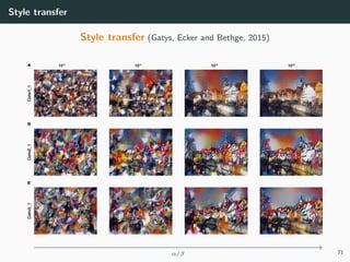
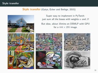
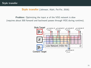
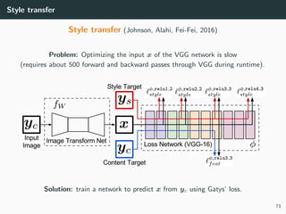
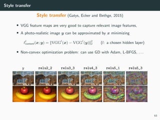
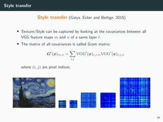
Style transfer (Gatys, Ecker and Bethge, 2015)
• VGG feature maps are very good to capture relevant image features,
• A photo-realistic image y can be approximated by x minimizing
l
content(x; y) = ||VGGl
(x) − VGGl
(y)||2
2 (l: a chosen hidden layer)
• Non-convex optimization problem: can use GD with Adam, L-BFGS, . . .
x = torch.rand(y.shape).cuda ()
x = nn.Parameter(x, requires_grad =True)
hy = VGGfeatures (y)[l]
optimizer = torch.optim.Adam ([x], lr =0.01)
f o r t i n range (0, T):
optimizer.zero_grad ()
hx = VGGfeatures(x)[l]
loss = ((hx - hy)**2).mean ()
loss.backward( retain_graph =True)
optimizer.step ()
62

71. Style transfer
Style transfer (Gatys, Ecker and Bethge, 2015)
• VGG feature maps are very good to capture relevant image features,
• A photo-realistic image y can be approximated by x minimizing
l
content(x; y) = ||VGGl
(x) − VGGl
(y)||2
2 (l: a chosen hidden layer)
• Non-convex optimization problem: can use GD with Adam, L-BFGS, . . .
63

72. Style transfer
Style transfer (Gatys, Ecker and Bethge, 2015)
• Texture/Style can be captured by looking at the covariances between all
VGG feature maps m and n of a same layer l.
• The matrix of all covariances is called Gram matrix:
Gl
(x)m,n =
i,j
VGGl
(x)i,j,mVGGl
(x)i,j,n
where (i, j) are pixel indices.
64

73. Style transfer
Style transfer (Gatys, Ecker and Bethge, 2015)
• Texture/Style can be captured by looking at the covariances between all
VGG feature maps m and n of a same layer l.
• The matrix of all covariances is called Gram matrix:
Gl
(x)m,n =
i,j
VGGl
(x)i,j,mVGGl
(x)i,j,n
where (i, j) are pixel indices.
64

74. Style transfer
Style transfer (Gatys, Ecker and Bethge, 2015)
• Texture/Style can be captured by looking at the covariances between all
VGG feature maps m and n of a same layer l.
• The matrix of all covariances is called Gram matrix:
Gl
(x)m,n =
i,j
VGGl
(x)i,j,mVGGl
(x)i,j,n
where (i, j) are pixel indices.
64

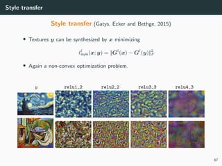
75. Style transfer
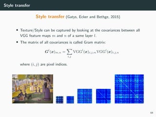
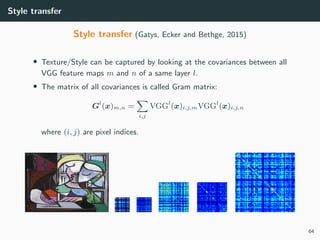
Style transfer (Gatys, Ecker and Bethge, 2015)
• Textures y can be synthesized by x minimizing
l
style(x; y) = ||Gl
(x) − Gl
(y)||2
F
• Again a non-convex optimization problem.
x = torch.rand(y.shape).cuda ()
x = nn.Parameter(x, requires_grad =True)
hy = VGGfeatures (y)[l]. view(C, W * H)
Gy = torch.mm(hy , hy.t())
f o r t i n range (0, T):
optimizer.zero_grad ()
hx = VGGfeatures(x)[l]. view(C, W * H)
Gx = torch.mm(hx , hx.t())
loss = ((Gx - Gy) ** 2).sum()
loss.backward( retain_graph =True)
optimizer.step ()
66

76. Style transfer
Style transfer (Gatys, Ecker and Bethge, 2015)
• Textures y can be synthesized by x minimizing
l
style(x; y) = ||Gl
(x) − Gl
(y)||2
F
• Again a non-convex optimization problem.
67

77. Style transfer
Style transfer (Gatys, Ecker and Bethge, 2015)
68

78. Style transfer
Style transfer (Gatys, Ecker and Bethge, 2015)
Style transfer: min
x
α l
content(x; yc)
match content at depth l
+ β
J
j=1
j
style(x; ys)
match texture from depth 1 to J
• Look for x such that
• its content corresponds to yc,
→ match VGG features at layer l (typically: l = 2, 3 or 4)
• its style corresponds to ys,
→ match VGG correlations at layers 1 to J (typically: J = 4 or 5)
• Again a non-convex optimization problem.
• Remark: no training data ⇒ not a ML algorithm,
→ this is just a simple CV technique relying on image features.
69

79. Style transfer
Style transfer (Gatys, Ecker and Bethge, 2015)
Style transfer: min
x
α l
content(x; yc)
match content at depth l
+ β
J
j=1
j
style(x; ys)
match texture from depth 1 to J
70

80. Style transfer
Style transfer (Gatys, Ecker and Bethge, 2015)
−−−−−−−−−−−−−−−−−−−−−−−−−−−−−−−−−−−−−−−−−−−−−−−−−−−−−−−−−→
α/β 71

81. Style transfer
Style transfer (Gatys, Ecker and Bethge, 2015)
Super easy to implement in PyTorch:
just sum all the losses with weights α and β!
But slow, about 15mins on DSMLP with GPU
for a 444 × 295 image.
72

82. Style transfer
Style transfer (Johnson, Alahi, Fei-Fei, 2016)
Problem: Optimizing the input x of the VGG network is slow
(requires about 500 forward and backward passes through VGG during runtime).
73

83. Style transfer
Style transfer (Johnson, Alahi, Fei-Fei, 2016)
Problem: Optimizing the input x of the VGG network is slow
(requires about 500 forward and backward passes through VGG during runtime).
Solution: train a network to predict x from yc using Gatys’ loss.
73

84. Style transfer
Style transfer (Johnson, Alahi, Fei-Fei, 2016)
min
θs
N
i=1
α l
content(x; yi
c)+β
J
j=1
j
style(x; ys)+ γ|| x||1
Total-Variation
where x = f(yi
c; θs)
• Add a Total-Variation term to encourage smoothness,
• Use a residual network with:
• 2 strided convolution to downsample,
• Several residual blocks (with shortcut connections),
• 2 fractionally strided convolutions to upsample.
• Trained on N = 80, 000 images of size 256 × 256 from MS COCO,
• One network has to be trained for each single target style ys,
• At test time, requires only one forward pass of this new network,
• Unlike Gatys’ method, this one is a ML algorithm.
74

85. Style transfer
Style transfer (Johnson, Alahi, Fei-Fei, 2016)
75

86. Questions?
That’s all folks!
Slides and images courtesy of
• Taegyun Jeon
• Justin Johnson
• Wikipedia
• Taegyun Jeon
• Fei-Fei Li
• Vijay Veerabadran
• Serena Yeung
• + all referenced articles
75