Download to read offline

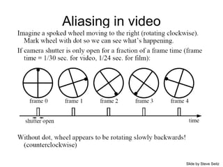
![Videos
[YouTube; JoinBuzzirk; phrancque]
Helicopter flying with no blades spinning !wheels spinning backwards](https://image.slidesharecdn.com/04cie552imagefilteringfrequency-200321060142/85/04-cie552-image_filtering_frequency-10-320.jpg)
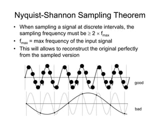
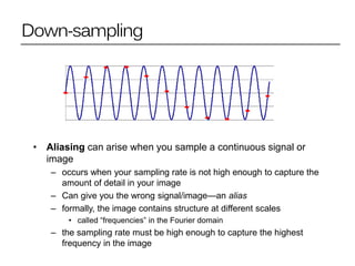
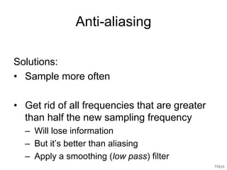
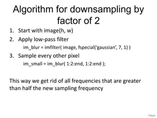
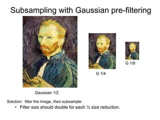
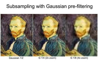
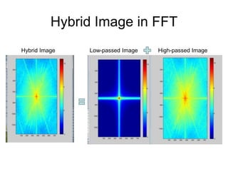
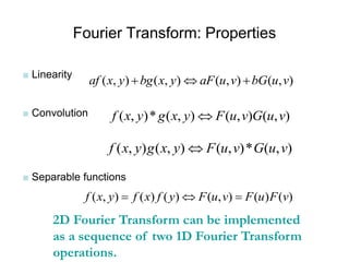
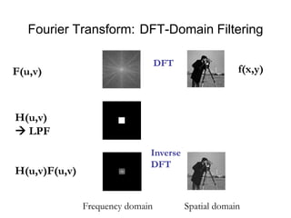
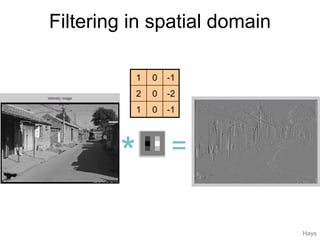
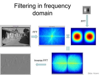
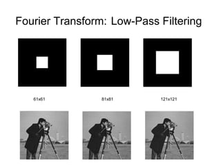
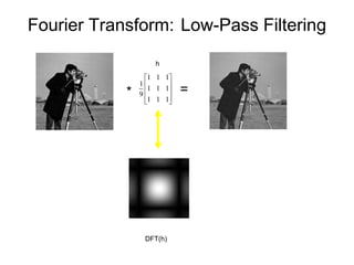
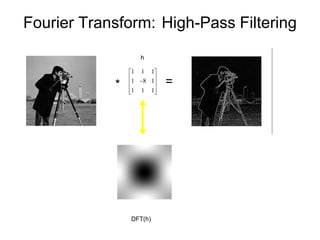
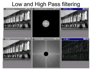
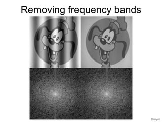
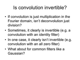
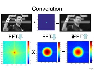
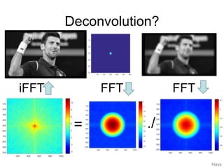
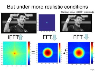
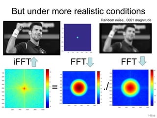

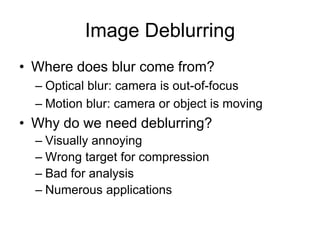
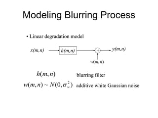
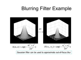
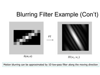
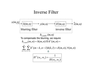
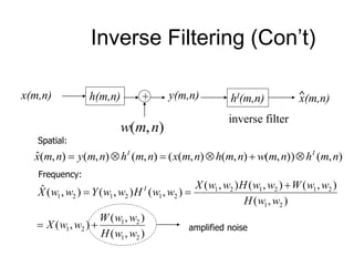
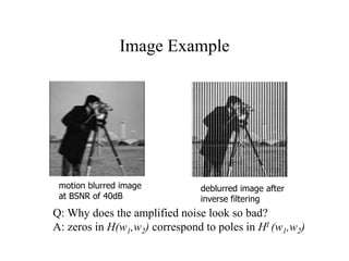
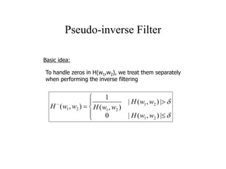
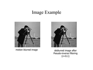
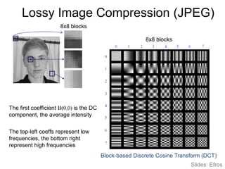
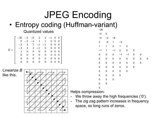
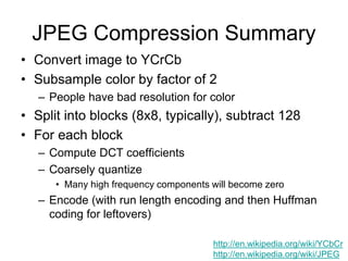


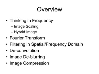
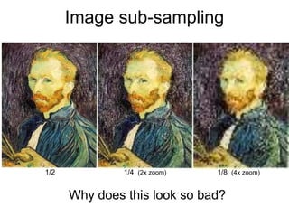
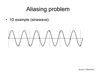
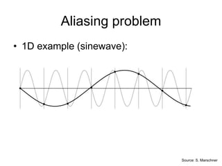
1. Image filtering can be performed in either the spatial or frequency domain using the Fourier transform. Low-pass filtering in the frequency domain removes high frequency components which can reduce aliasing when downsampling images. 2. Deconvolution aims to reverse the effects of blurring by dividing the Fourier transform of an image by the Fourier transform of the blurring filter, but this amplifies noise. Pseudoinverse filtering handles zeros in the blurring filter to improve results. 3. JPEG compression transforms image blocks to the frequency domain via DCT, quantizes and discards high frequency coefficients, and entropy codes the results to achieve high compression ratios with minimal perceived quality loss.