Download to read offline

![Convolution
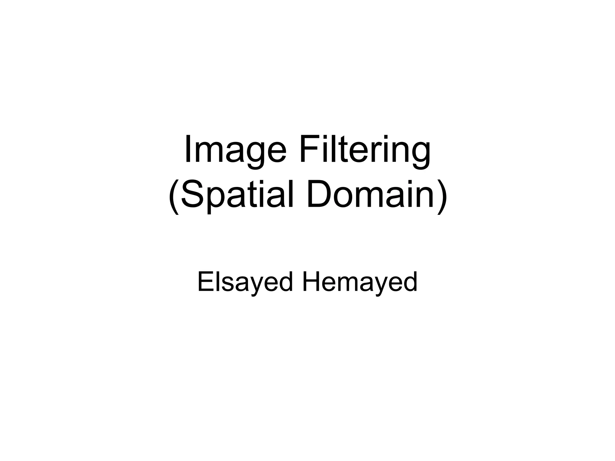
• Convolution of two functions is defined as
– In the discrete case is:
( )* ( ) ( ) ( )f x h x f h x d
[ ]* [ ] [ ] [ ]
m
f n h n f m h n m
](https://image.slidesharecdn.com/03cie552imagefilteringspatial-200321055729/75/03-cie552-image_filtering_spatial-3-2048.jpg)
![• In the 2D discrete case Convolution is
defined as:
is called a linear filter1 2[ , ]h n n
Convolution – 2D](https://image.slidesharecdn.com/03cie552imagefilteringspatial-200321055729/75/03-cie552-image_filtering_spatial-5-2048.jpg)
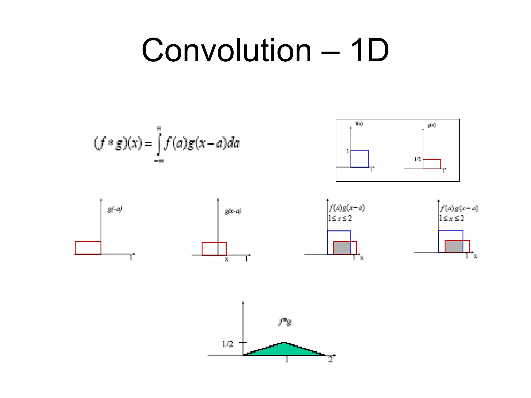
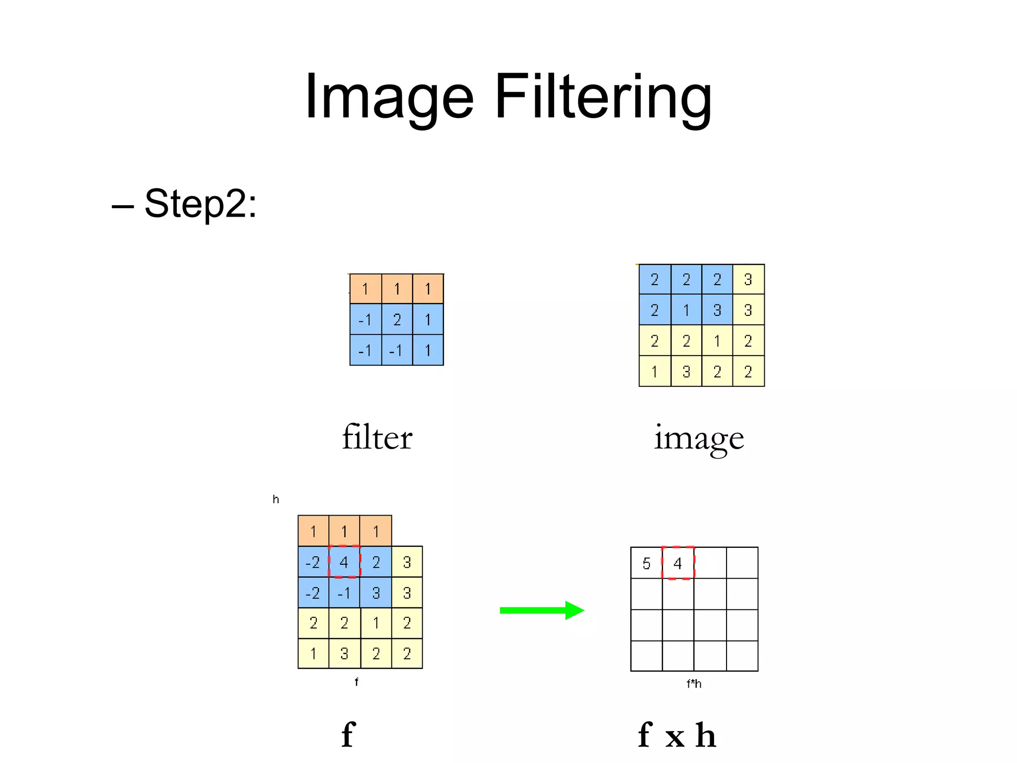
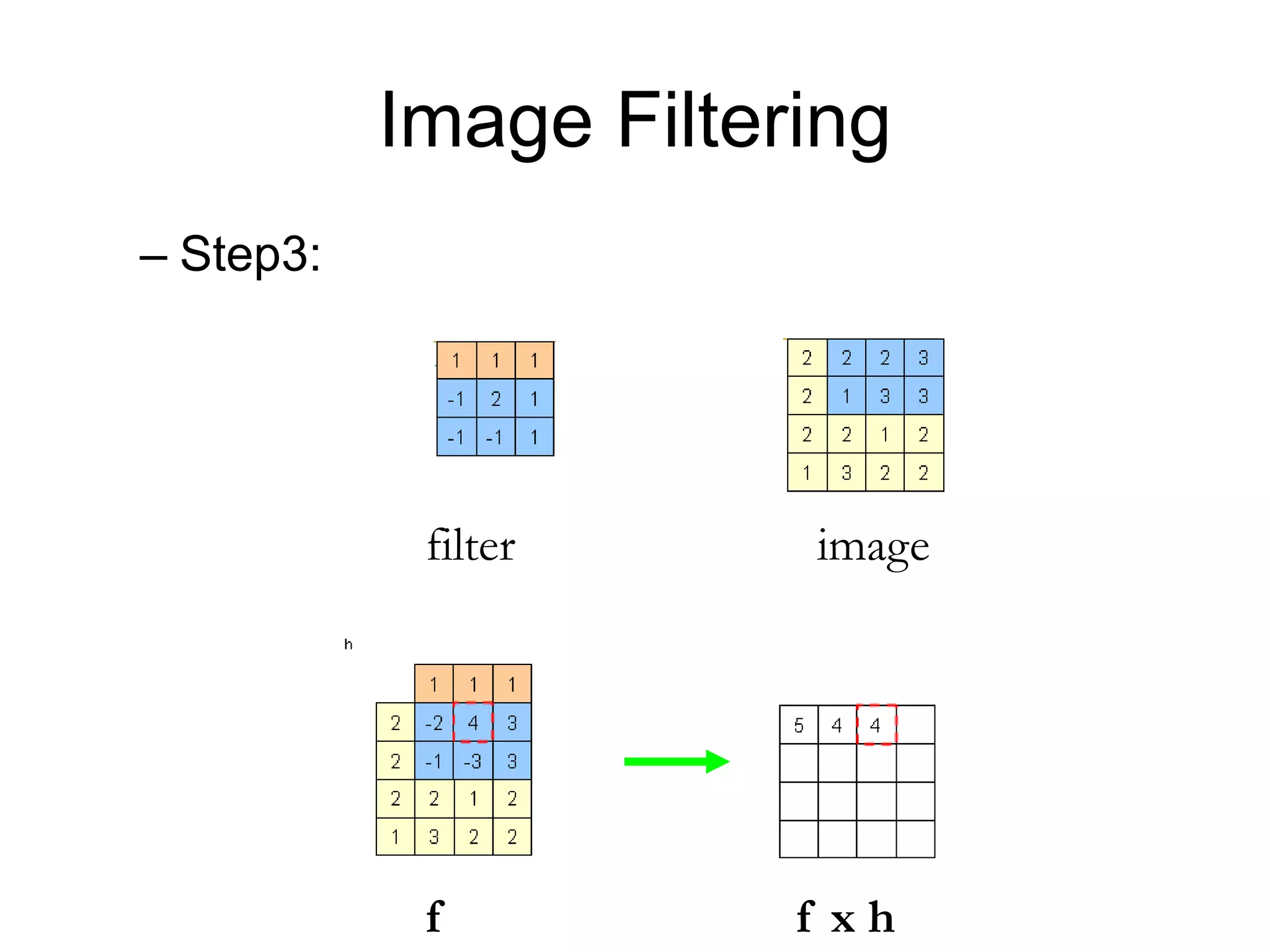
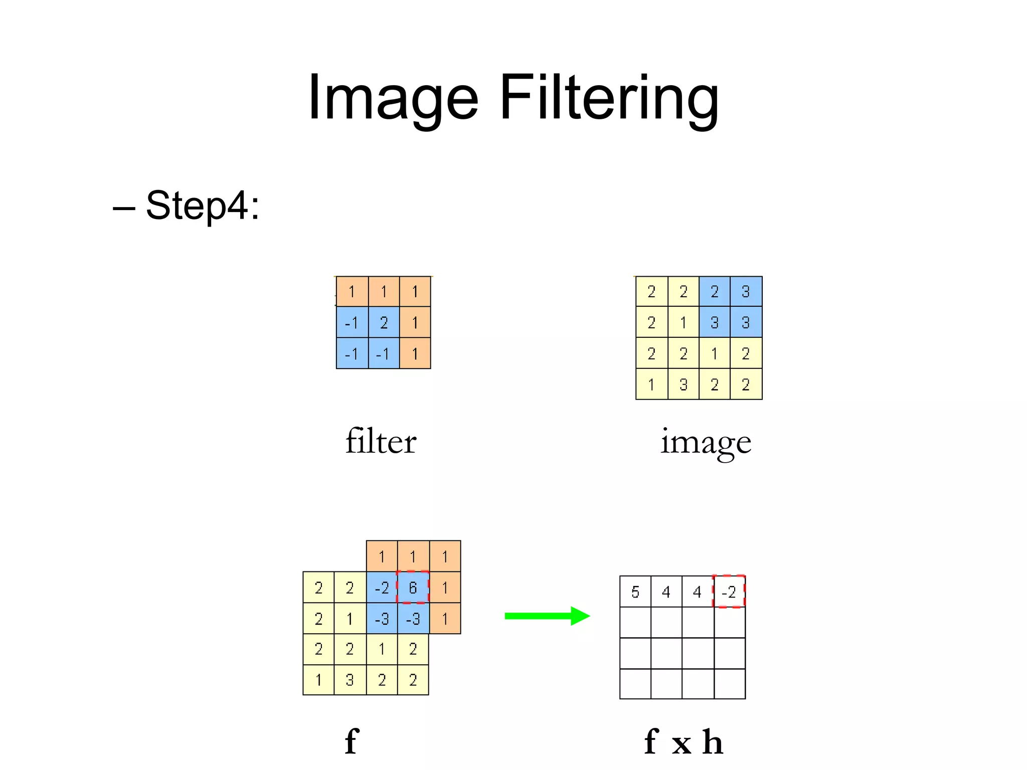
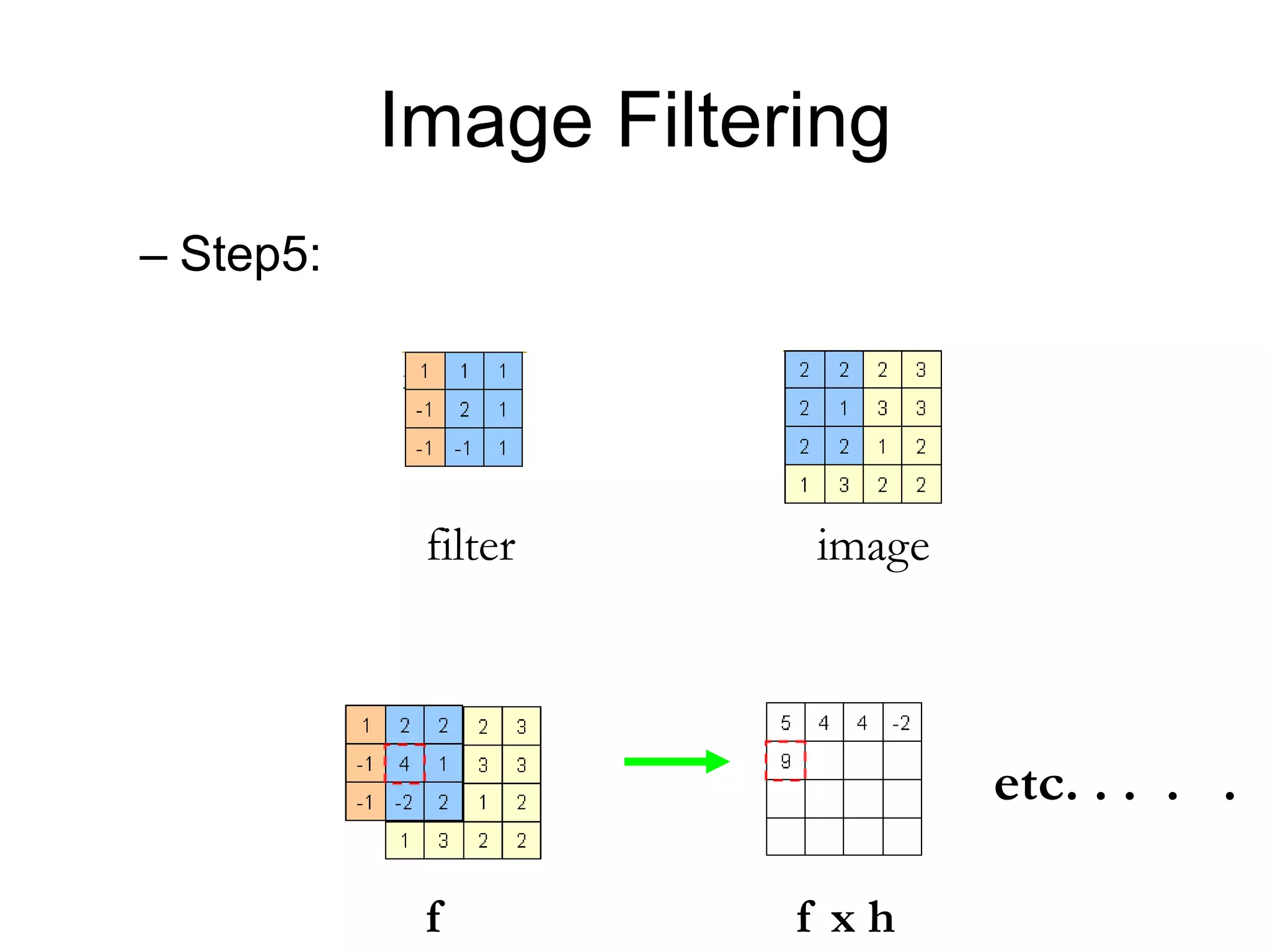
![Image filtering• Image filtering:
– Compute function of local neighborhood at each position
],[],[],[
,
lnkmIlkfnmh
lk
I=imagef=filterh=output
2d coords=m,n2d coords=k,l
[ ] [ ]
[ ]](https://image.slidesharecdn.com/03cie552imagefilteringspatial-200321055729/75/03-cie552-image_filtering_spatial-6-2048.jpg)
![Correlation and Convolution
• 2d correlation
],[],[],[
,
lnkmIlkfnmh
lk
James Hays
e.g., h = scipy.signal.correlate2d(f,I)](https://image.slidesharecdn.com/03cie552imagefilteringspatial-200321055729/75/03-cie552-image_filtering_spatial-7-2048.jpg)
![Correlation and Convolution
• 2d correlation
• 2d convolution
],[],[],[
,
lnkmIlkfnmh
lk
],[],[],[
,
lnkmIlkfnmh
lk
Convolution is the same as correlation with a 180° rotated filter kernel.
Correlation and convolution are identical when the filter kernel is symmetric
James Hays
e.g., h = scipy.signal.correlate2d(f,I)
e.g., h = scipy.signal.convolve2d(f,I)](https://image.slidesharecdn.com/03cie552imagefilteringspatial-200321055729/75/03-cie552-image_filtering_spatial-8-2048.jpg)
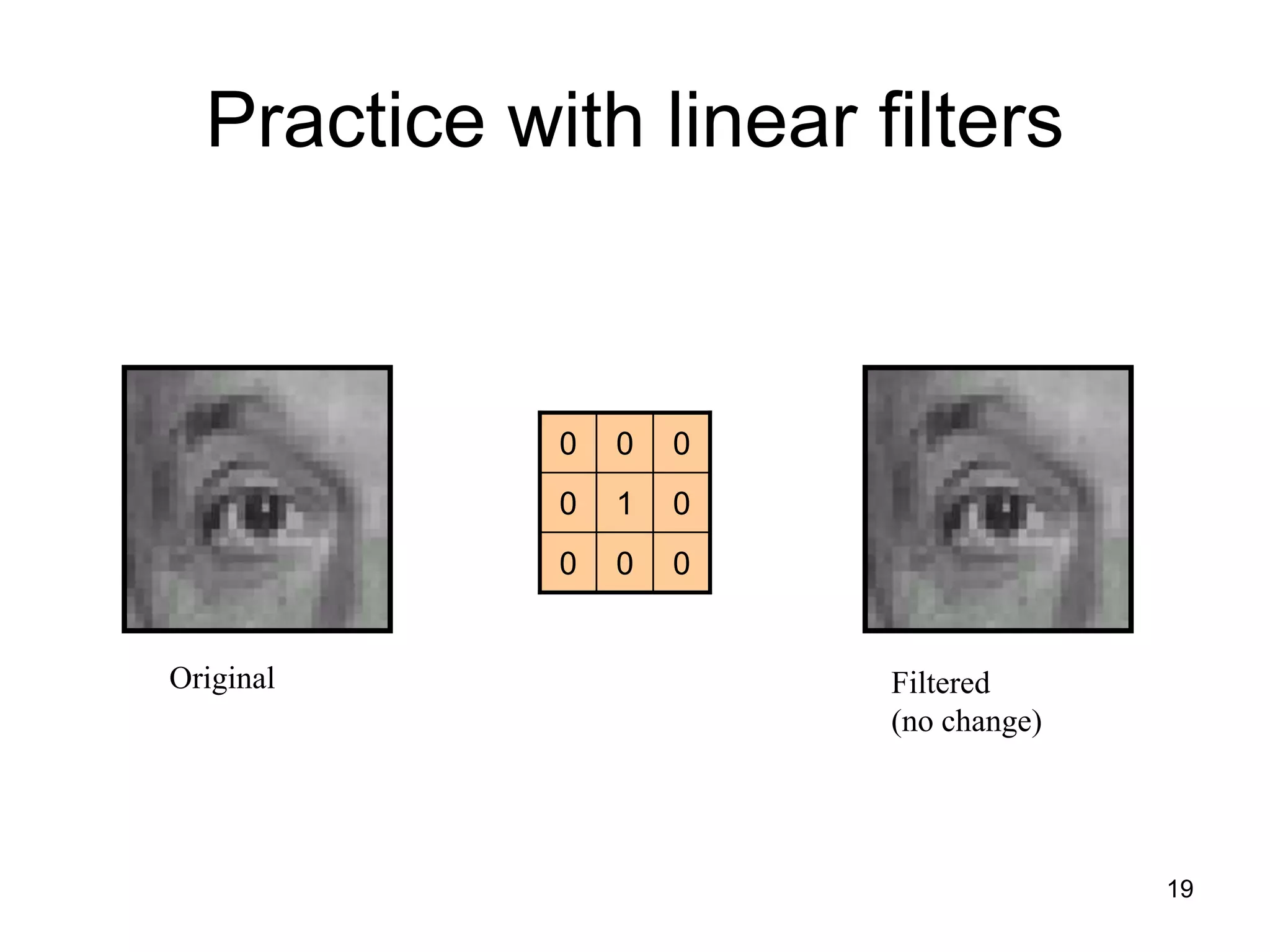
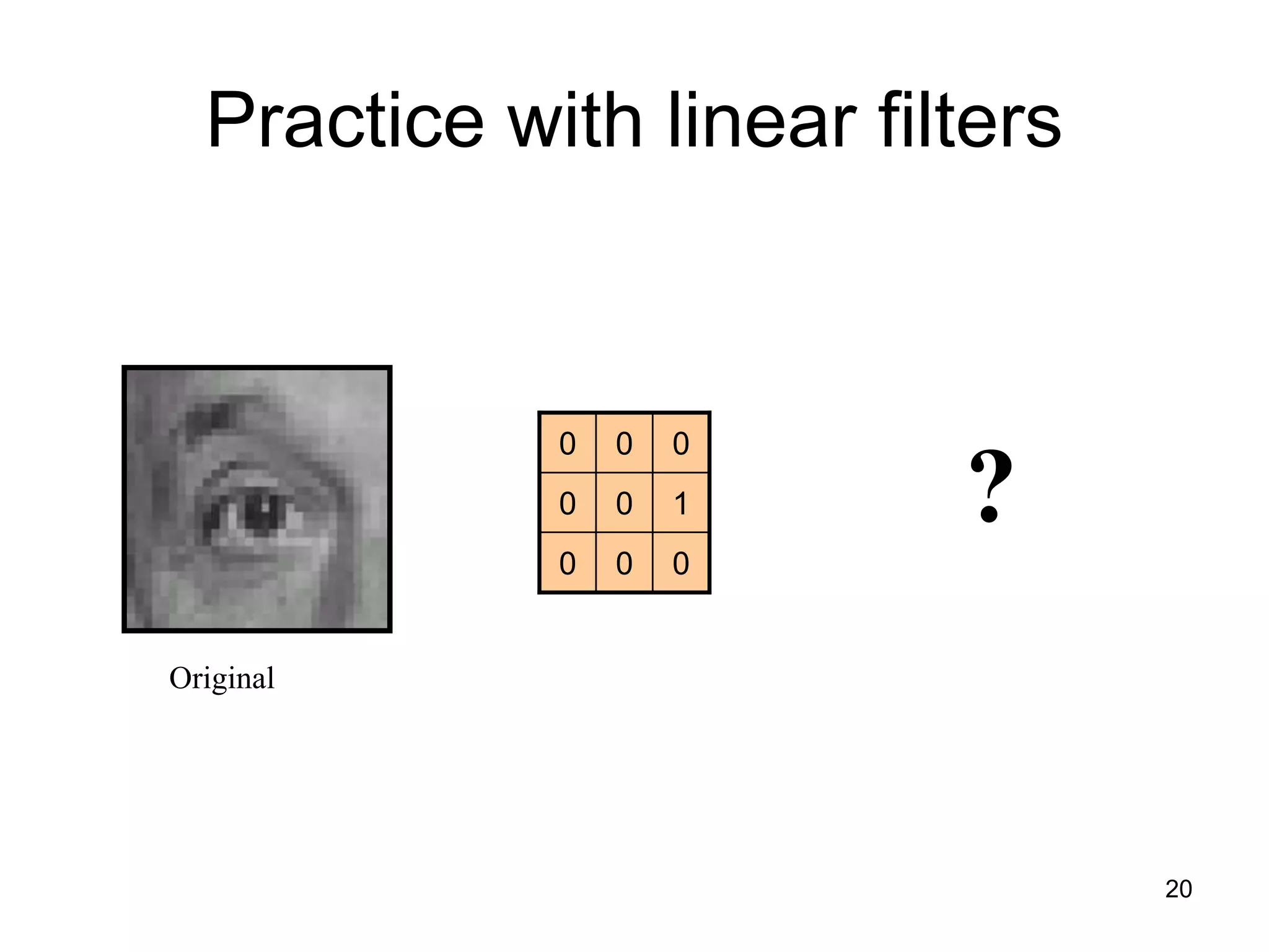
![Image filtering
• Image filtering:
– Compute function of local neighborhood at each
position
• Really important!
– Enhance images
• Denoise, resize, increase contrast, etc.
– Extract information from images
• Texture, edges, distinctive points, etc.
– Detect patterns
• Template matching
],[],[],[
,
lnkmIlkfnmh
lk
James Hays](https://image.slidesharecdn.com/03cie552imagefilteringspatial-200321055729/75/03-cie552-image_filtering_spatial-14-2048.jpg)
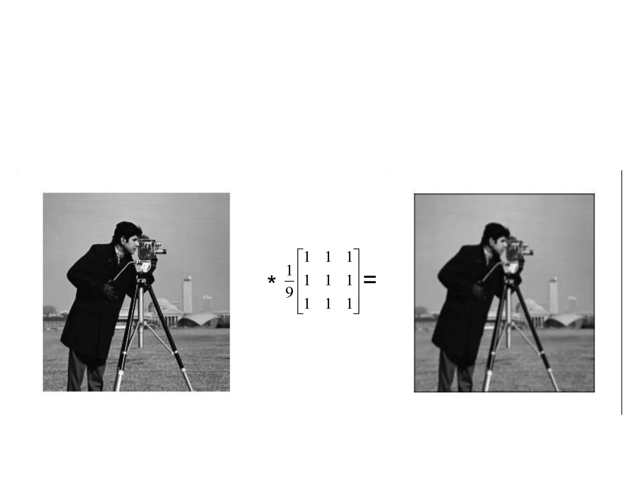
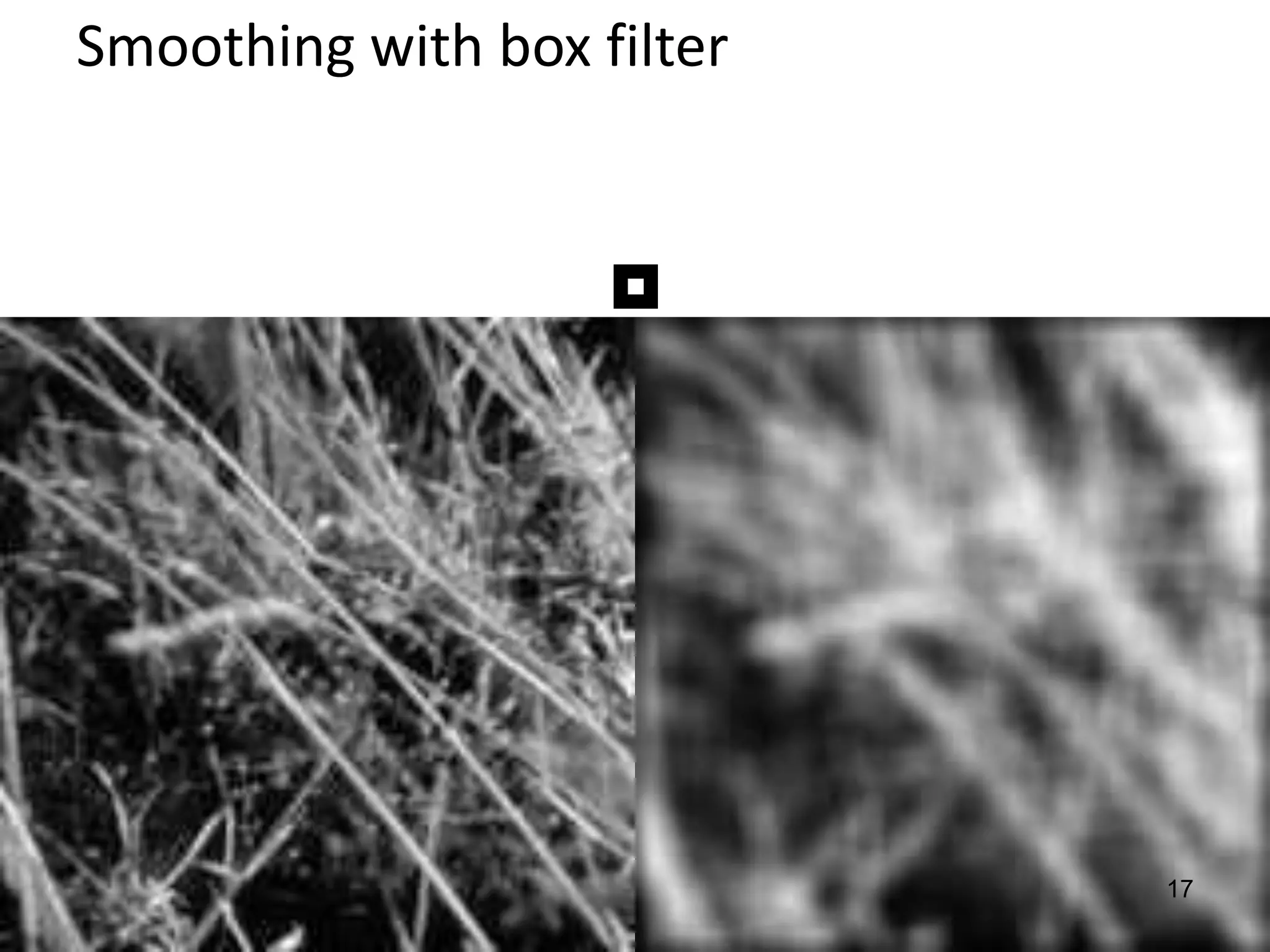
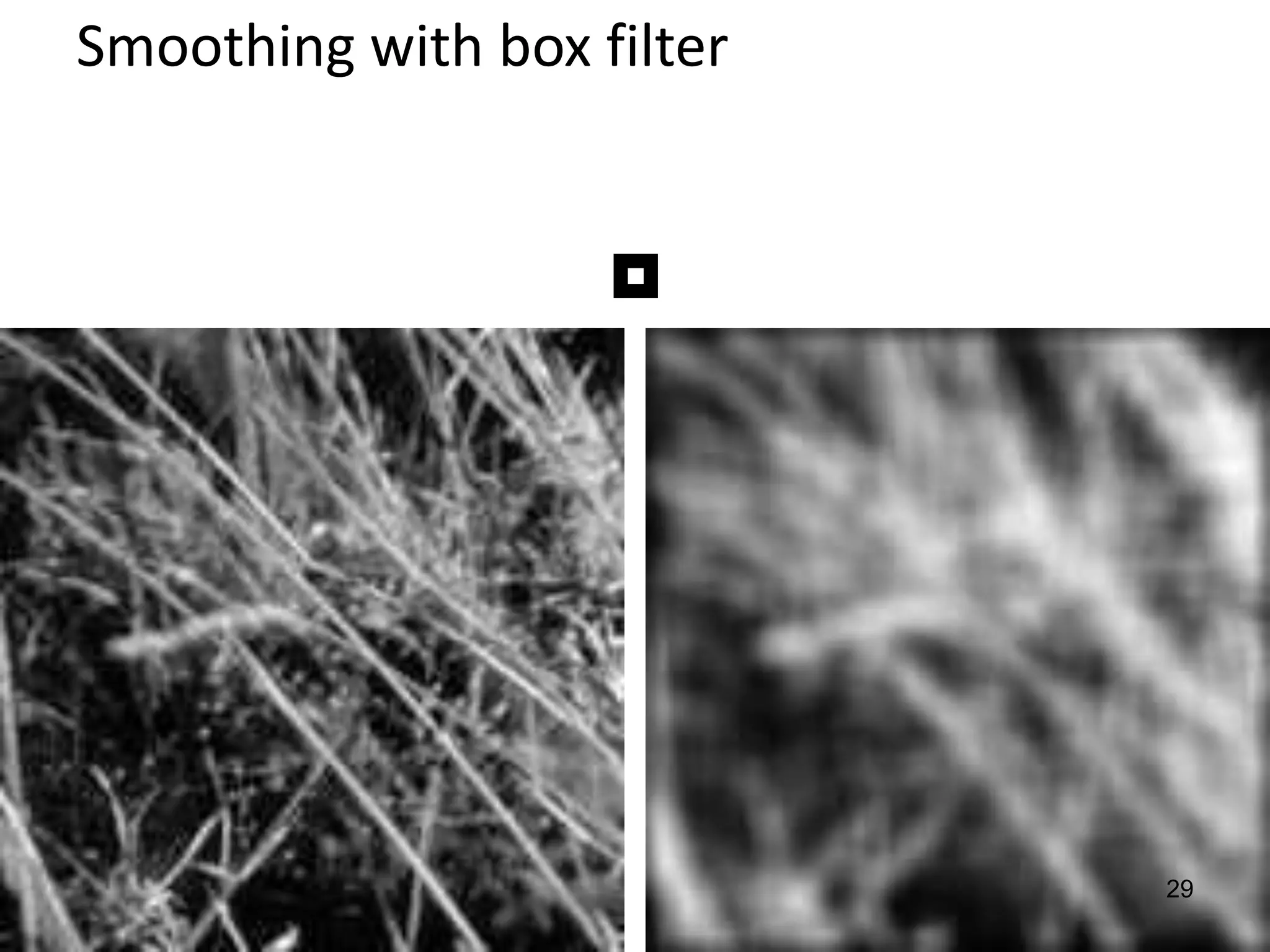
![What does it do?
• Replaces each pixel with
an average of its
neighborhood
• Achieve smoothing effect
(remove sharp features)
111
111
111
],[g
Box Filter
15](https://image.slidesharecdn.com/03cie552imagefilteringspatial-200321055729/75/03-cie552-image_filtering_spatial-15-2048.jpg)


![>> f = D[ 57:117, 107:167 ]
Expect response ‘peak’ in middle of I
>> I = correlate2d( D, f, ‘same’ )
f
61 x 61
D (275 x 175 pixels)
I
Response
peak
Hmm…
That didn’t work – why not?
+
Correct
location
[Thanks to Robert Collins @ Penn State]
Template Matching](https://image.slidesharecdn.com/03cie552imagefilteringspatial-200321055729/75/03-cie552-image_filtering_spatial-43-2048.jpg)
![Correlation
],[],[],[
,
lnkmIlkfnmh
lk
e.g., h = scipy.signal.correlate2d(f,I)
As brightness in I increases, the response
in h will increase, as long as f is positive.
Overall brighter regions will give higher
correlation response -> not useful!](https://image.slidesharecdn.com/03cie552imagefilteringspatial-200321055729/75/03-cie552-image_filtering_spatial-44-2048.jpg)
![OK, so let’s subtract the mean
>> f = D[ 57:117, 107:167 ]
>> f2 = f – np.mean(f)
>> D2 = D – np.mean(D)
Now zero centered.
Score is higher only when dark parts
match and when light parts match.
>> I2 = correlate2d( D2, f2, ‘same’ )
f2
61 x 61
D2 (275 x 175 pixels)
I2](https://image.slidesharecdn.com/03cie552imagefilteringspatial-200321055729/75/03-cie552-image_filtering_spatial-45-2048.jpg)
![What happens with convolution?
>> f = D[ 57:117, 107:167 ]
>> f2 = f – np.mean(f)
>> D2 = D – np.mean(D)
>> I2 = convolve2d( D2, f2, ‘same’ )
f2
61 x 61
D2 (275 x 175 pixels)
I2](https://image.slidesharecdn.com/03cie552imagefilteringspatial-200321055729/75/03-cie552-image_filtering_spatial-47-2048.jpg)

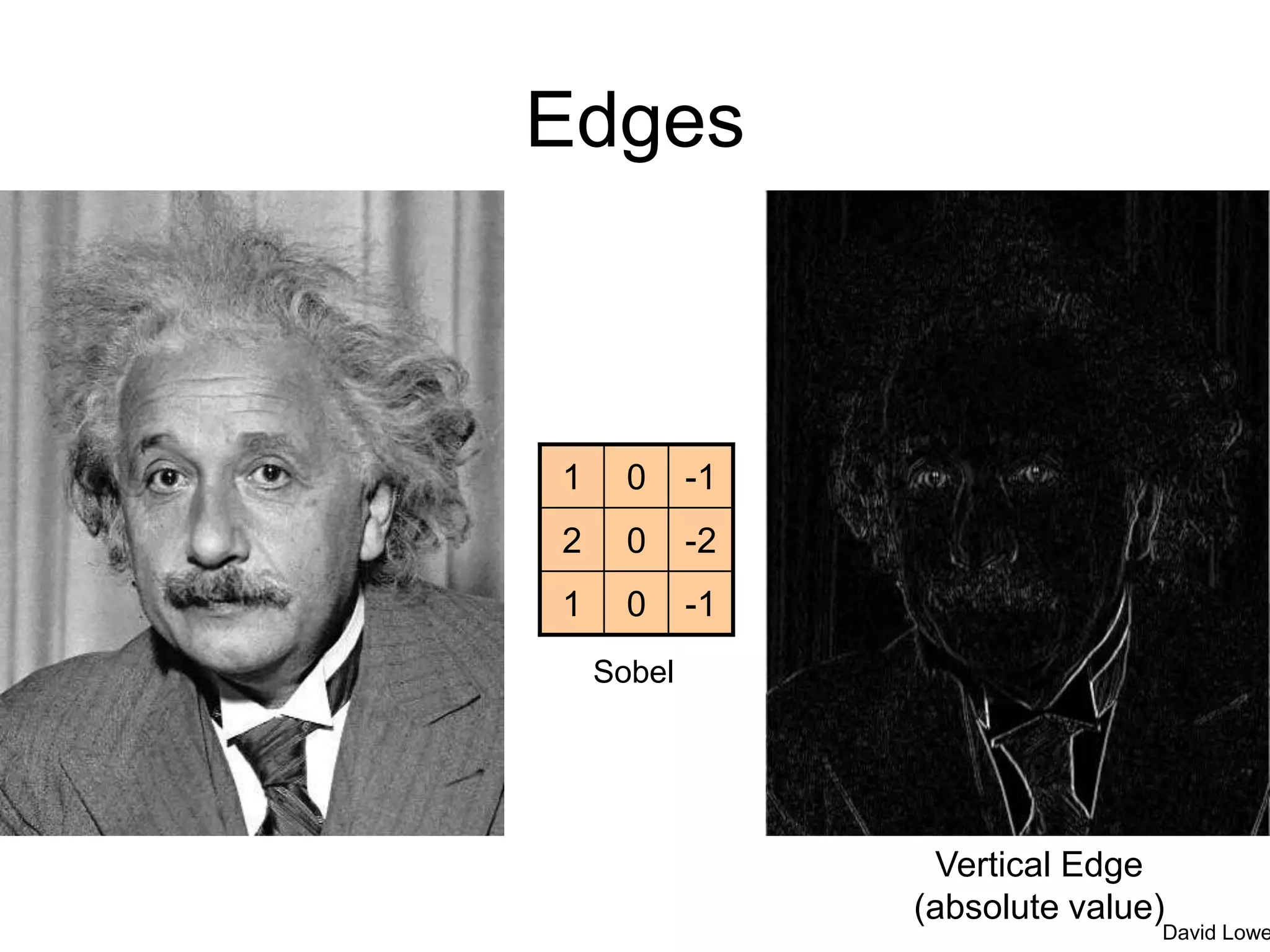
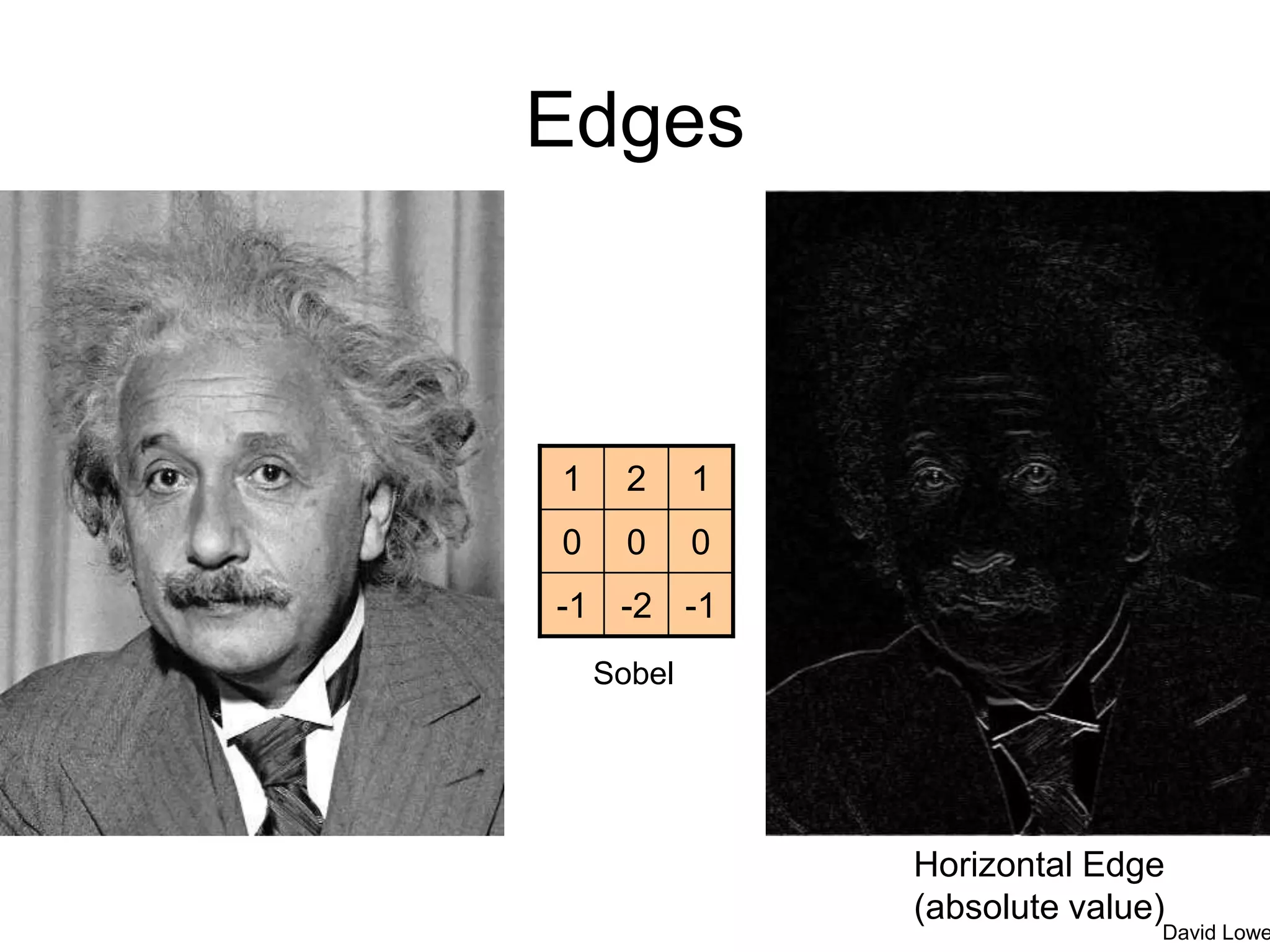
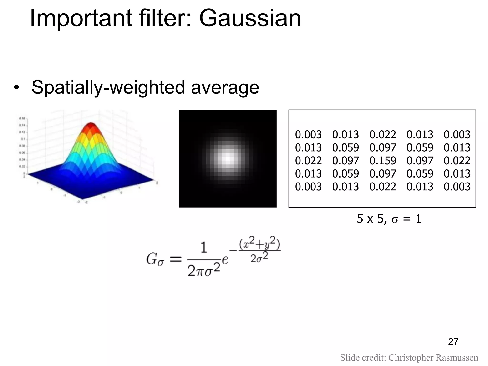
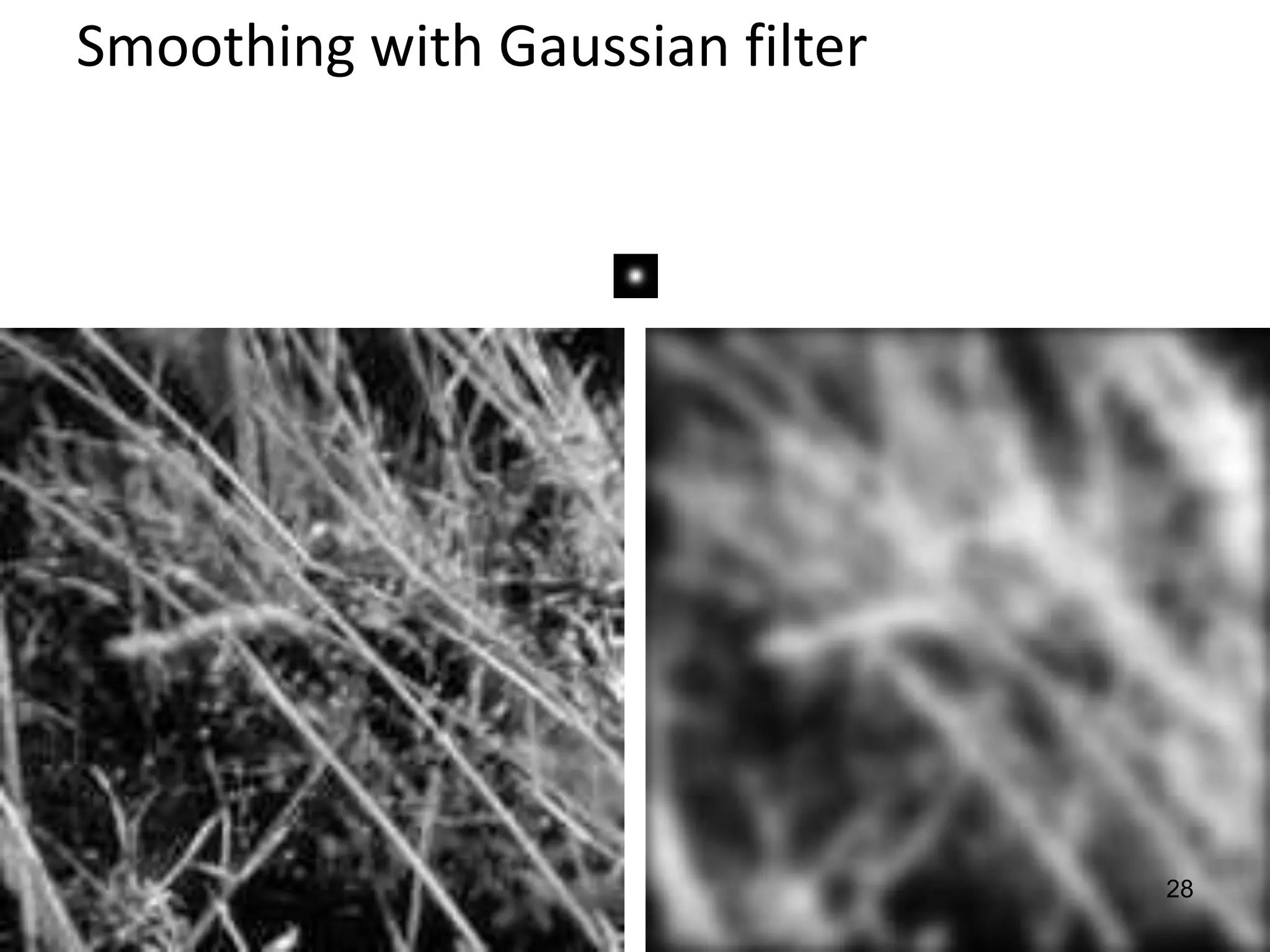
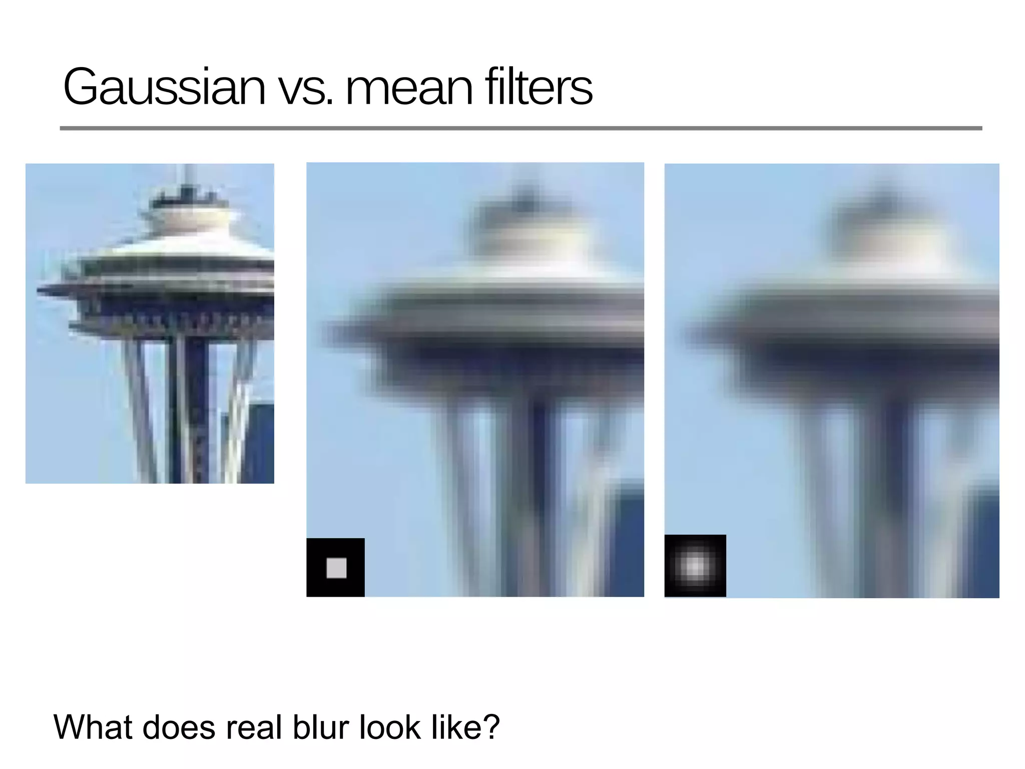
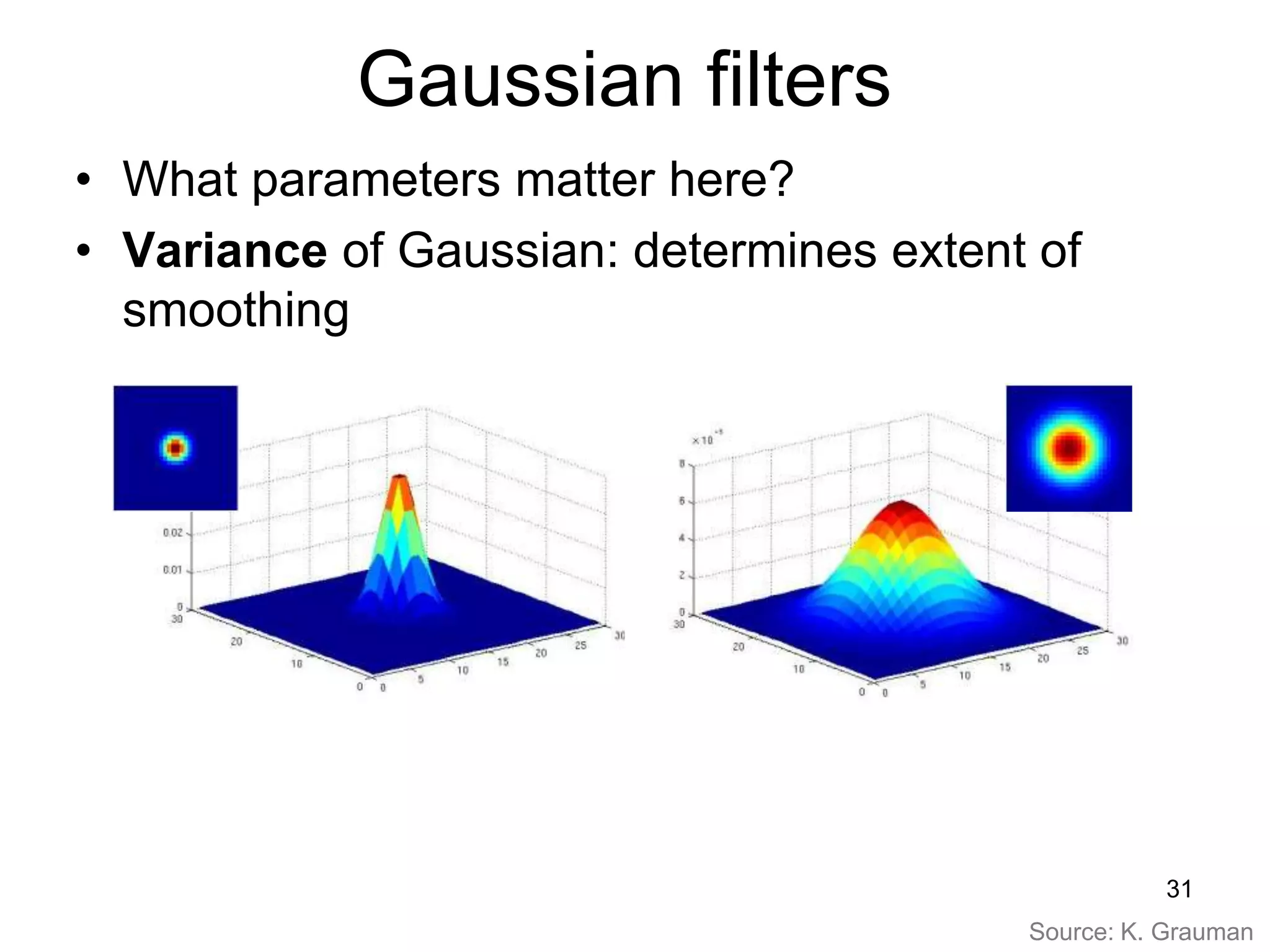
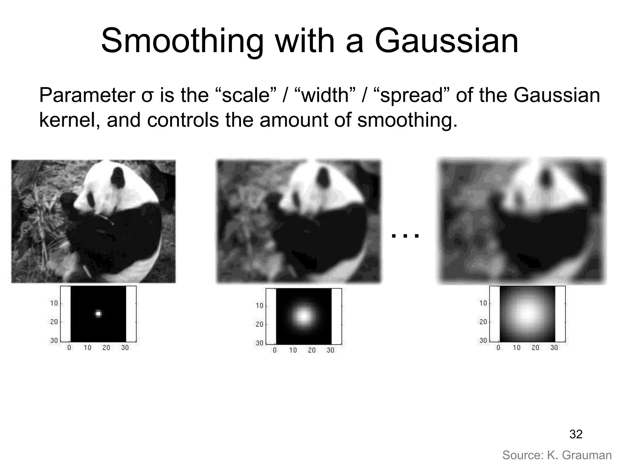
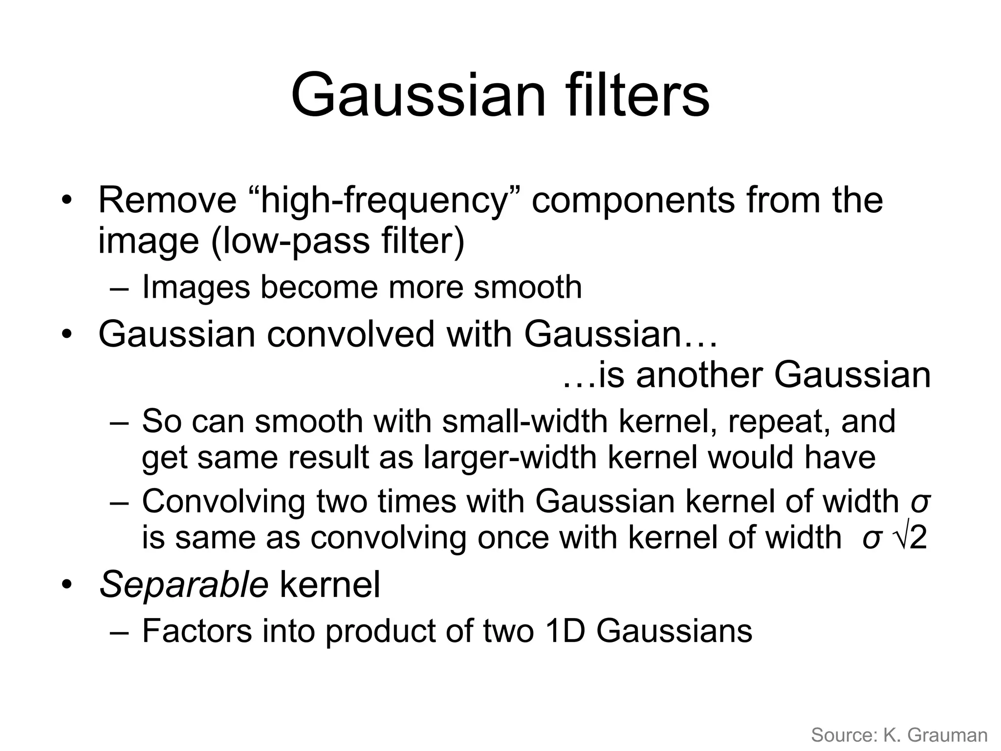
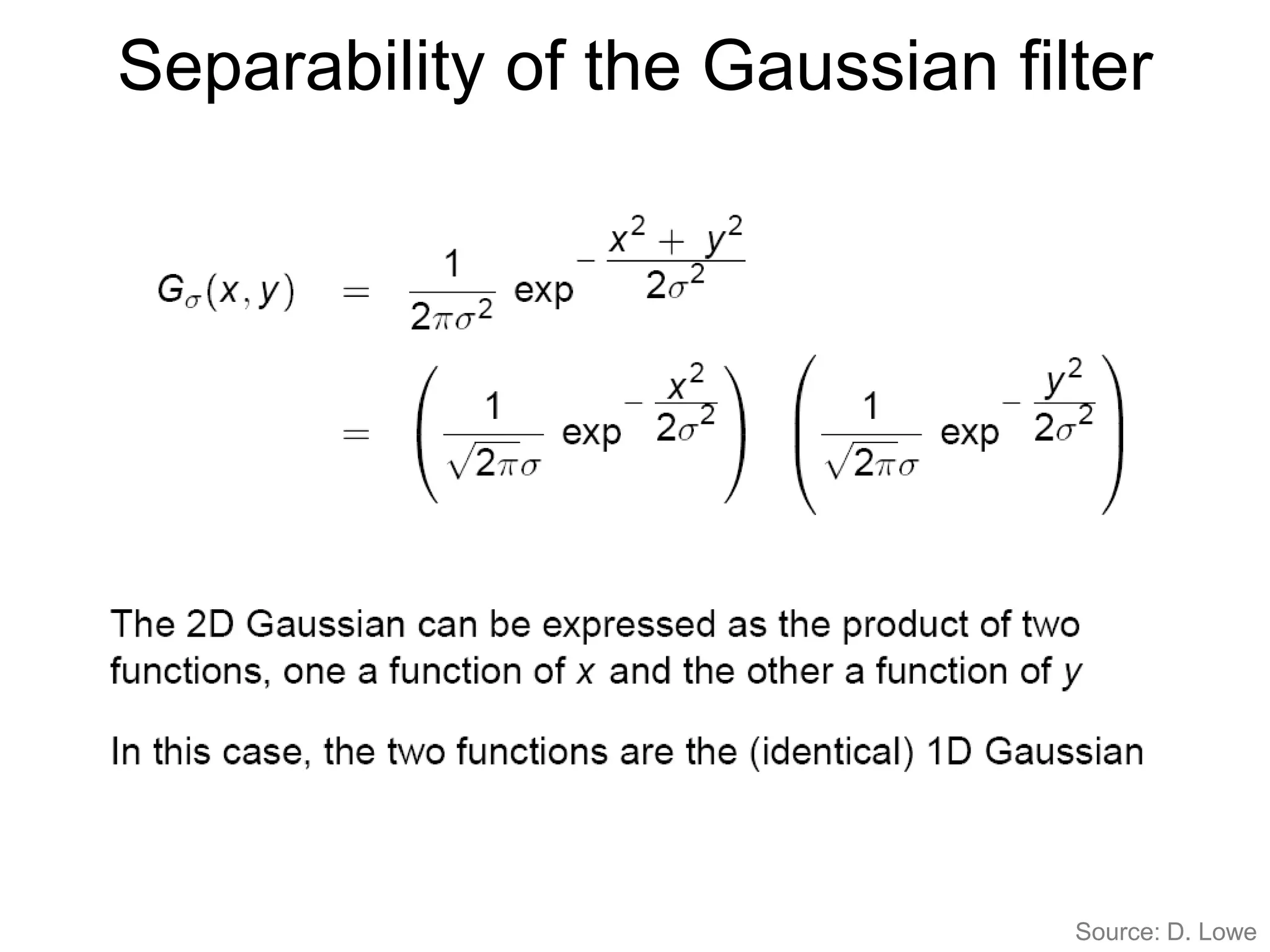
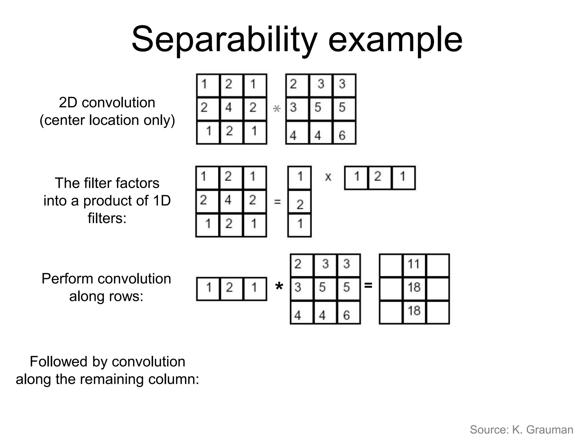
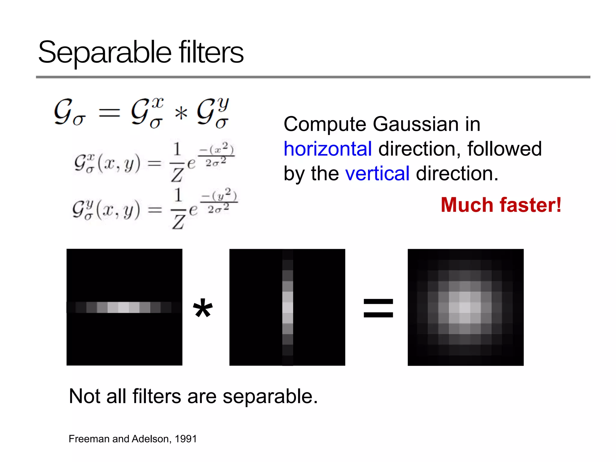
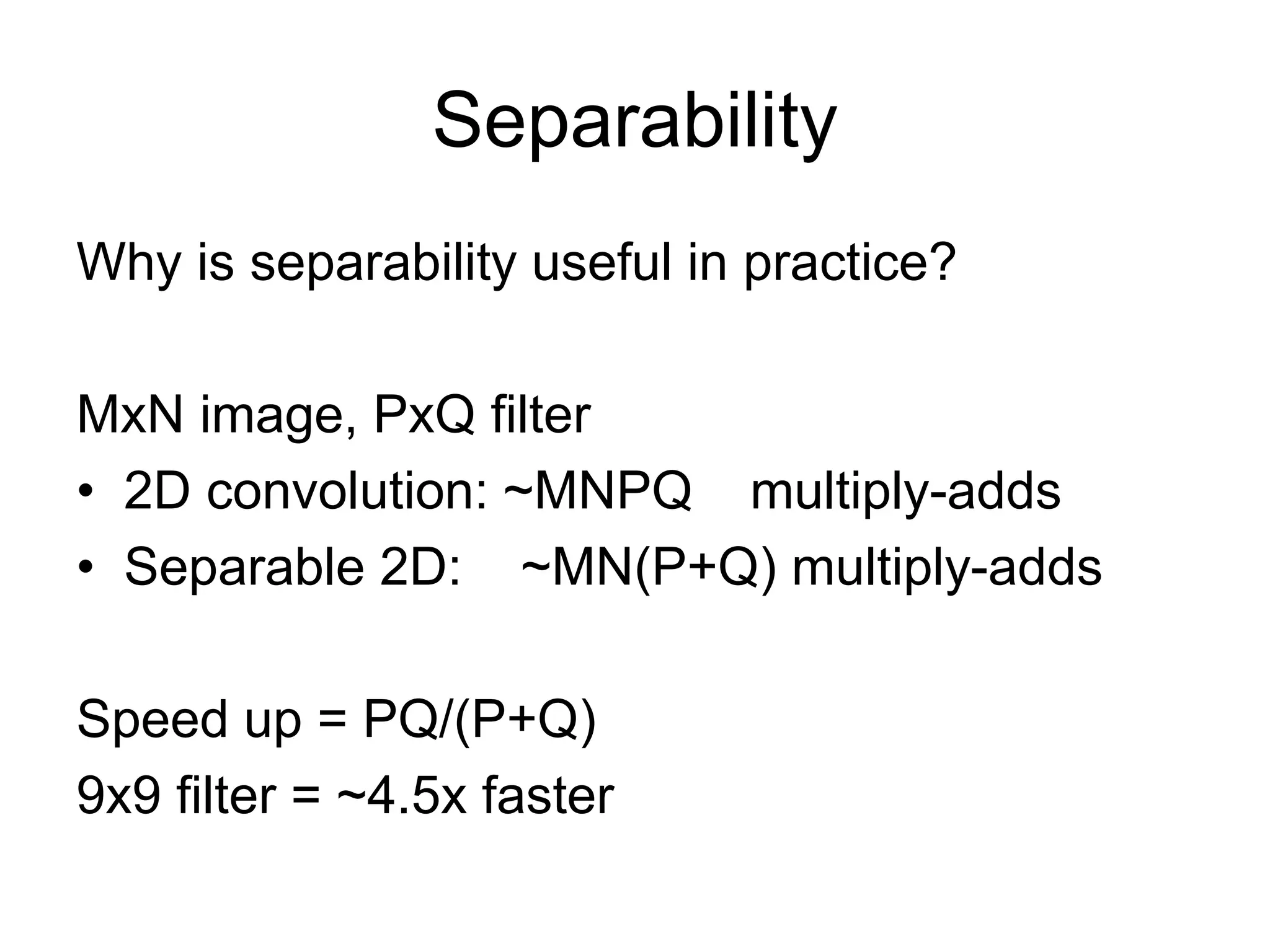
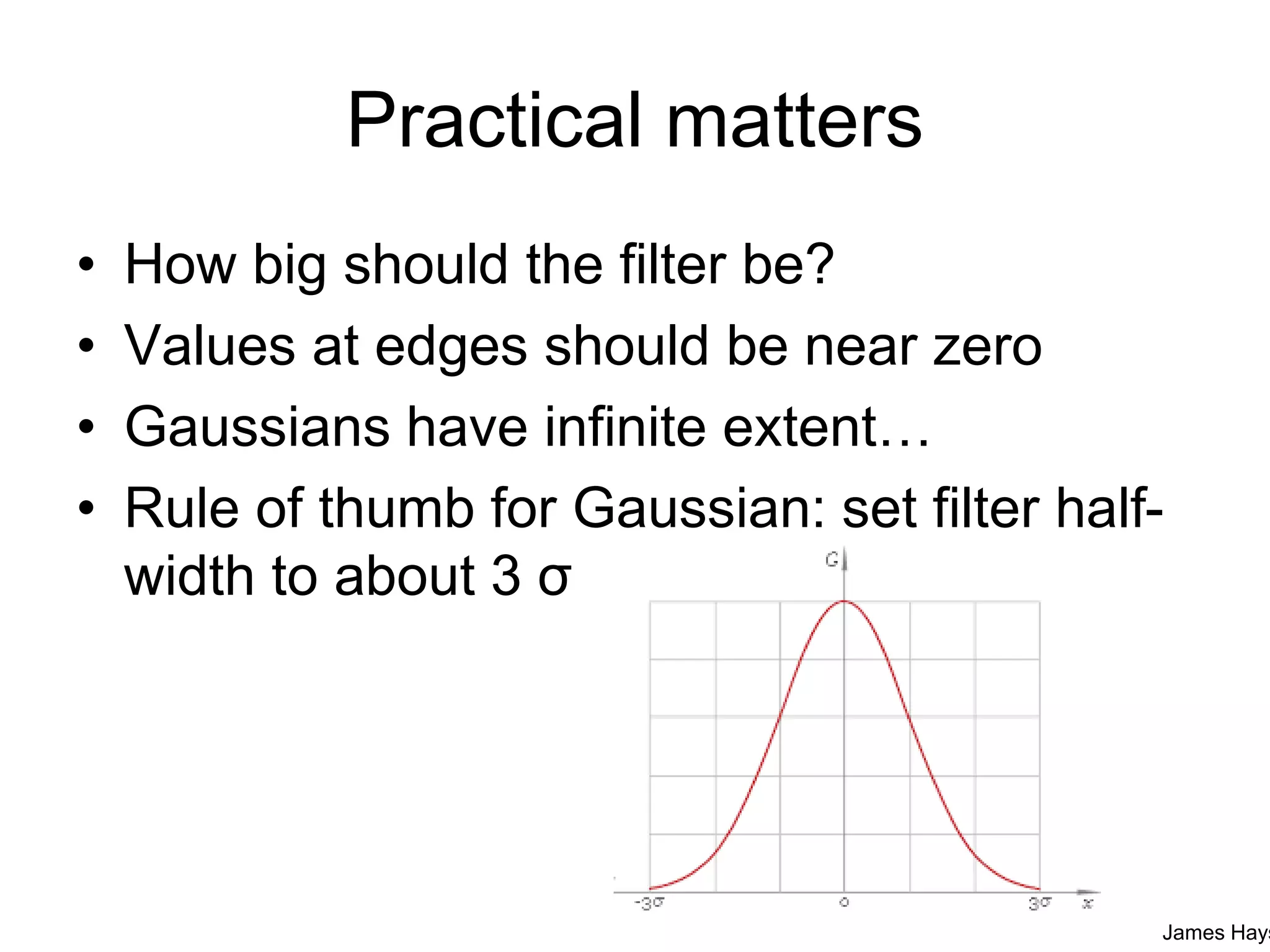
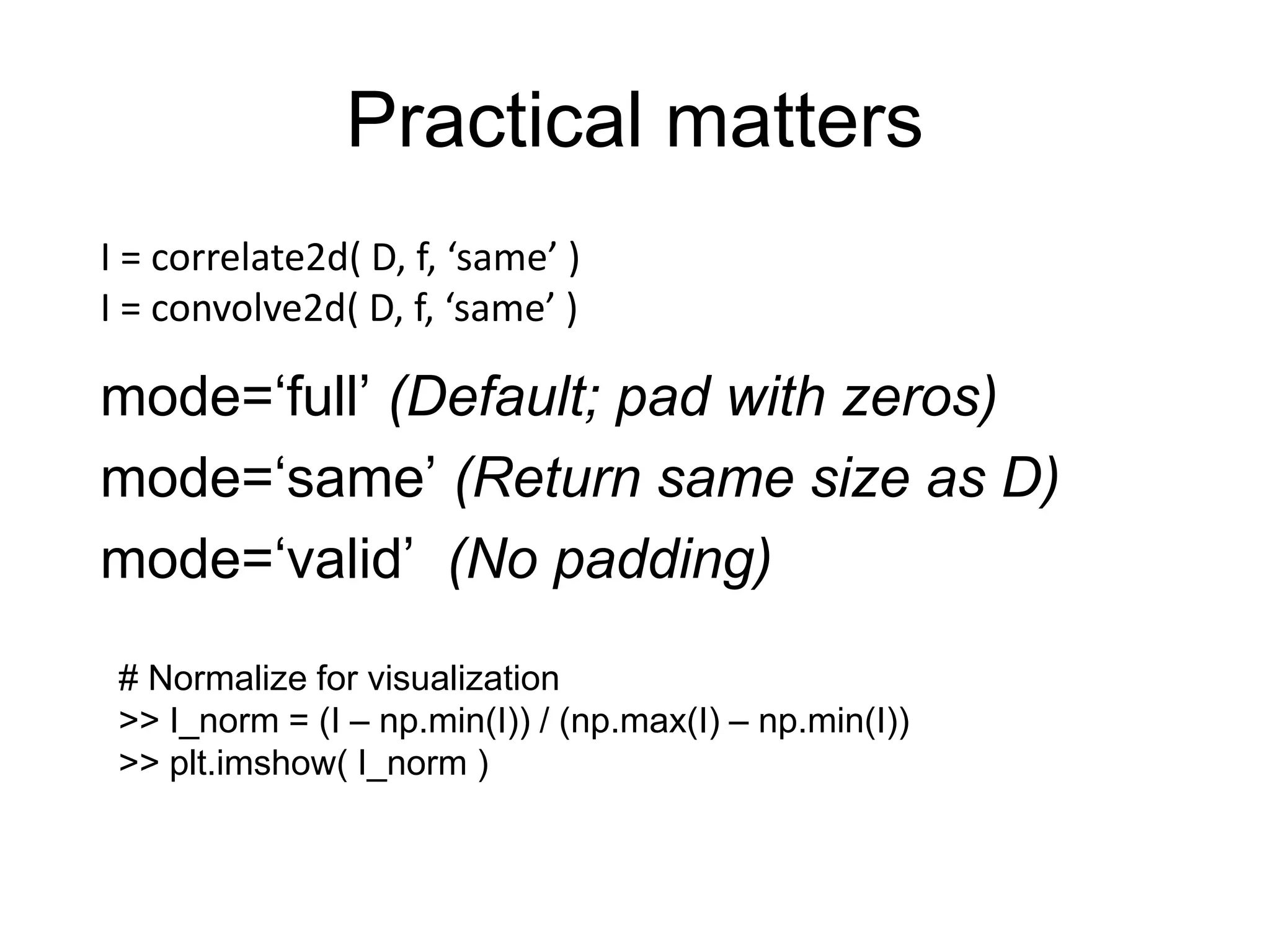
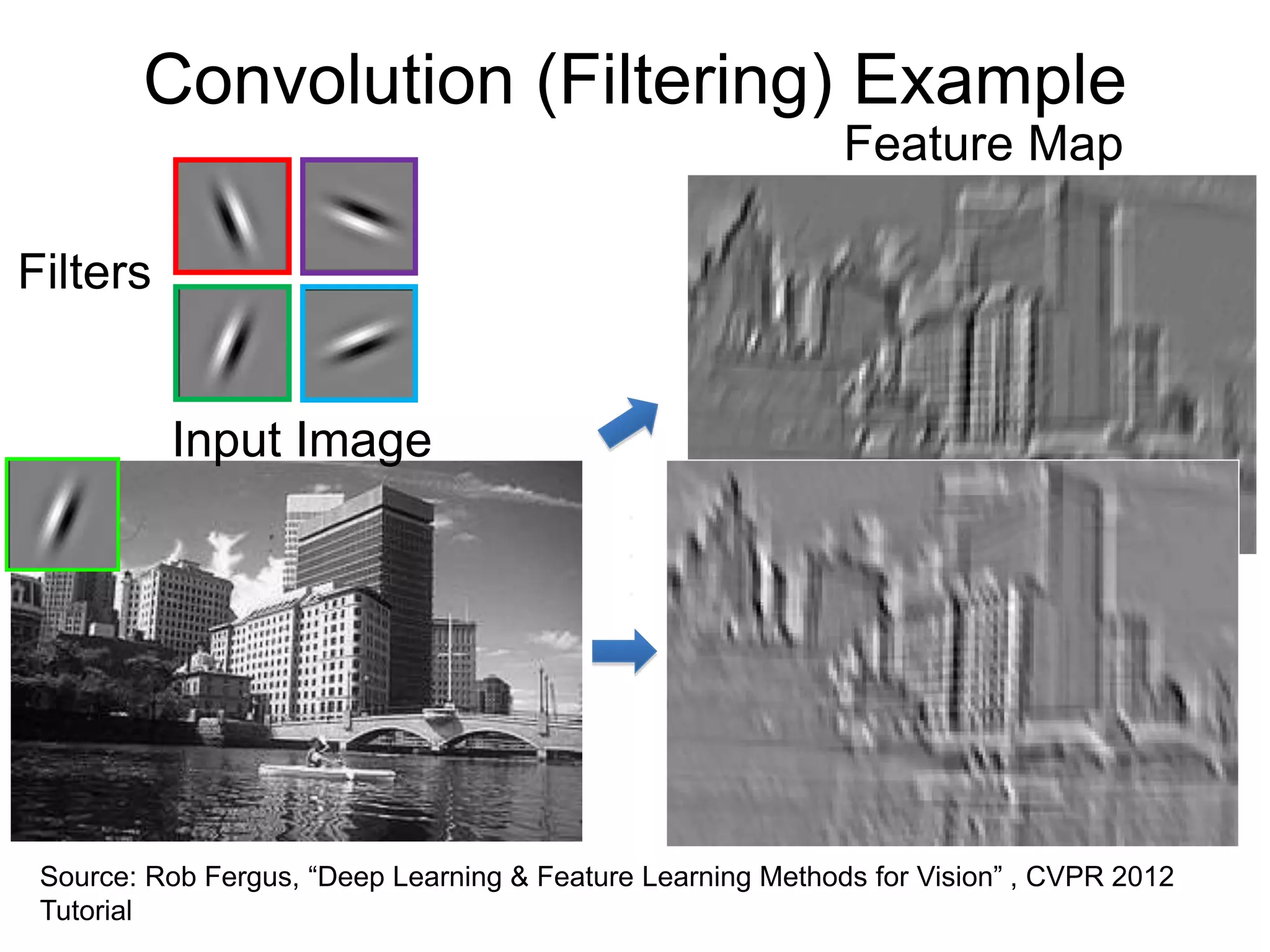
1. Image filtering involves applying convolution operations to images using filters like box filters and Gaussian filters. This smooths images by averaging pixel neighborhoods. 2. Gaussian filters are commonly used to smooth images as they produce realistic blurring effects. The amount of smoothing depends on the Gaussian's variance parameter. 3. Template matching uses correlation or convolution to find regions in an image that match a template pattern. It is commonly used for tasks like object detection.