Download as PDF, PPTX

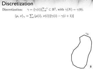
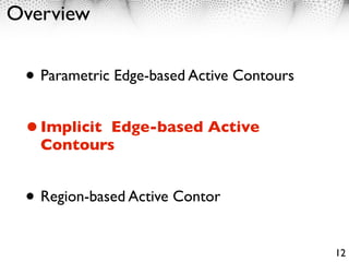
![Intrinsic Curve Evolutions
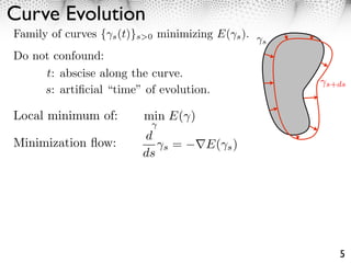
E( ) only depends on { (t) t [0, 1]}.
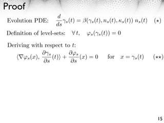
Intrinsic energy E: evolution along the normal
s
d
⇥s (t) = (⇥s (t), ns (t), ⇤s (t)) ns (t) ns
ds
speed normal
s (t)
Normal: ns (t) =
|| s (t)||
1
Curvature: ⇥s (t) = ns (t), s (t)⇥
|| s (t)||2
6](https://image.slidesharecdn.com/course-mesh-active-contours-121213054004-phpapp01/85/Mesh-Processing-Course-Active-Contours-10-320.jpg)
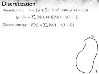
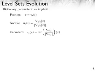
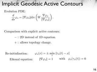
![Level Sets
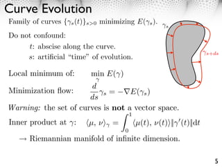
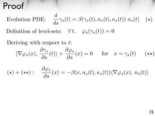
Level-set curve representation:
s (x) 0
{ s (t) t [0, 1]} = x R ⇥s (x) = 0 .
2
Example: circle of radius r s (x) = ||x x0 || s
Example: square of radius r s (x) = ||x x0 || s
s (x) 0](https://image.slidesharecdn.com/course-mesh-active-contours-121213054004-phpapp01/85/Mesh-Processing-Course-Active-Contours-21-320.jpg)
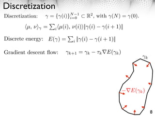
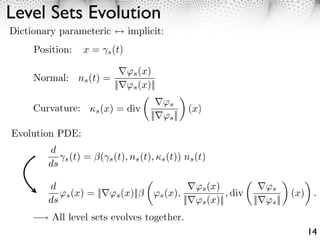
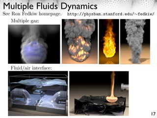
![Level Sets
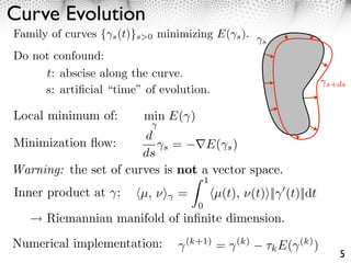
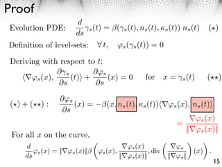
Level-set curve representation:
s (x) 0
{ s (t) t [0, 1]} = x R ⇥s (x) = 0 .
2
Example: circle of radius r s (x) = ||x x0 || s
Example: square of radius r s (x) = ||x x0 || s
s (x) 0
Union of domains: s = min( 1
s, s)
2
Intersection of domains: s = max( 1
s, s)
2
s (x) 0
s = min( 1
s, s)
2](https://image.slidesharecdn.com/course-mesh-active-contours-121213054004-phpapp01/85/Mesh-Processing-Course-Active-Contours-22-320.jpg)
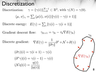
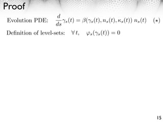
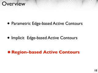
![Level Sets
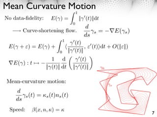
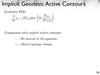
Level-set curve representation:
s (x) 0
{ s (t) t [0, 1]} = x R ⇥s (x) = 0 .
2
Example: circle of radius r s (x) = ||x x0 || s
Example: square of radius r s (x) = ||x x0 || s
s (x) 0
Union of domains: s = min( 1
s, s)
2
Intersection of domains: s = max( 1
s, s)
2
s (x) 0
Popular choice: (signed) distance to a curve
⇥s (x) = ± min || s (t) x||
t
infinite number of mappings s s.
s = min( 1
s, s)
2](https://image.slidesharecdn.com/course-mesh-active-contours-121213054004-phpapp01/85/Mesh-Processing-Course-Active-Contours-23-320.jpg)
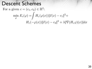
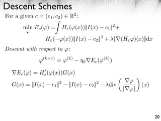
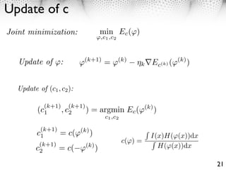
![Energy Depending on Region
Optimal segmentation [0, 1]2 = c
:
min L1 ( ) + L2 ( c
) + R( ) R( ) = | |
Data Regularization
fidelity
Chan-Vese binary model: L1 ( ) = |I(x) c1 |2 dx
More general models
19](https://image.slidesharecdn.com/course-mesh-active-contours-121213054004-phpapp01/85/Mesh-Processing-Course-Active-Contours-34-320.jpg)
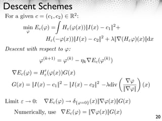
![Energy Depending on Region
Optimal segmentation [0, 1]2 = c
:
min L1 ( ) + L2 ( c
) + R( ) R( ) = | |
Data Regularization
fidelity
Chan-Vese binary model: L1 ( ) = |I(x) c1 |2 dx
More general models
Level set implementation: = {x (x) > 0}
2 x H(x)
Smoothed Heaviside: H (x) = atan
⇥ x
L1 ( ) ⇥ L( ) = H ( (x))||I(x) c1 ||2 dx
R( ) R( ) = ||⇥(H )(x)||dx
19](https://image.slidesharecdn.com/course-mesh-active-contours-121213054004-phpapp01/85/Mesh-Processing-Course-Active-Contours-35-320.jpg)
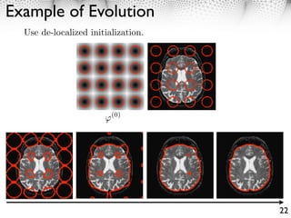
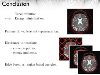

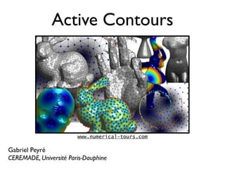
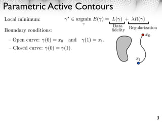
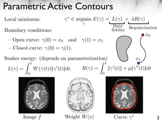
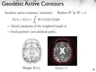
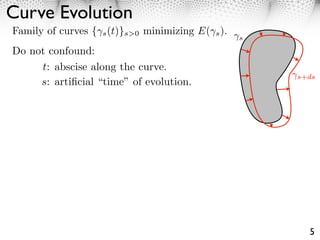
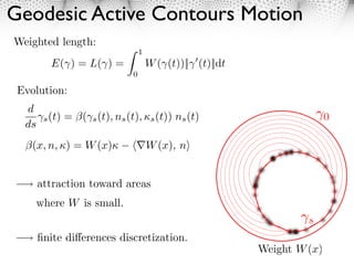
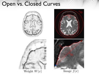
(1) Active contours, or snakes, are parametric or geometric active contour models used for edge detection and image segmentation. (2) Parametric active contours represent curves explicitly through parameterization, while implicit active contours represent curves as the zero level set of a higher dimensional function. (3) Active contours evolve to minimize an energy functional comprising an internal regularization term and an external image-based term, converging to object boundaries or other image features.