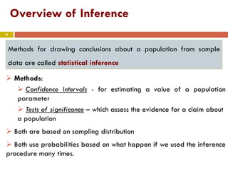
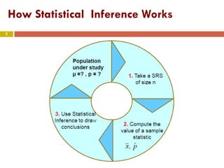
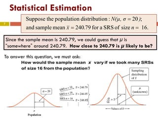
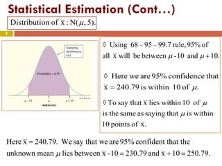
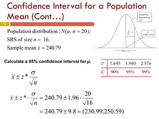
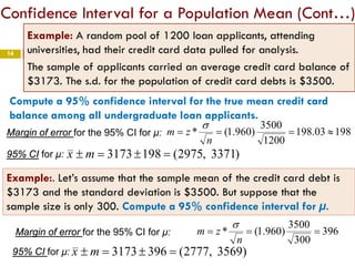
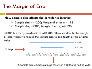
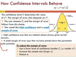
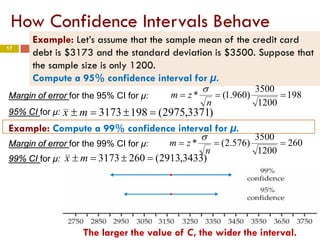
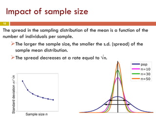
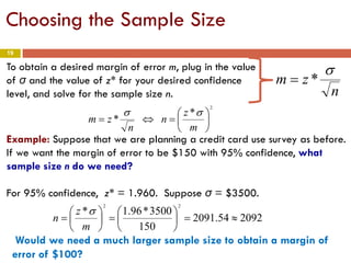
Chapter 6 part1- Introduction to Inference-Estimating with Confidence (Introduction to Inference, Estimating with Confidence, Inference, Statistical Confidence, Confidence Intervals, Confidence Interval for a Population Mean, Choosing the Sample Size)
Introduction to Inference, Estimating with Confidence, Inference, Statistical Confidence, Confidence Intervals, Confidence Interval for a Population Mean, Choosing the Sample Size
This document discusses key concepts in research methods and biostatistics, including hypothesis testing, random error, p-values, and confidence intervals. It explains that hypothesis testing involves determining if study findings reflect chance or a true effect. The p-value represents the probability of observing results as extreme or more extreme than what was observed by chance alone. A p-value less than 0.05 indicates statistical significance. Confidence intervals provide a range of values that are likely to contain the true population parameter.
This document discusses key concepts in statistics for engineers and scientists such as point estimates, properties of good estimators, confidence intervals, and the t-distribution. A point estimate is a single numerical value used to estimate a population parameter from a sample. A good estimator must be unbiased, consistent, and relatively efficient. A confidence interval provides a range of values that is likely to contain the true population parameter based on the sample data and confidence level. The t-distribution is similar to the normal distribution but has greater variance and depends on degrees of freedom. Examples are provided to demonstrate how to calculate confidence intervals for means using the normal and t-distributions.
Chapter 6 part2-Introduction to Inference-Tests of Significance, Stating Hyp...nszakir
Mathematics, Statistics, Introduction to Inference, Tests of Significance, The Reasoning of Tests of Significance, Stating Hypotheses, Test Statistics, P-values, Statistical Significance, Test for a Population Mean, Two-Sided Significance Tests and Confidence Intervals
Discrete and continuous probability distributions ppt @ bec domsBabasab Patil
The document discusses various probability distributions including discrete and continuous distributions. It covers the binomial, hypergeometric, Poisson, and normal distributions. It provides the characteristics and formulas for each distribution and examples of how to calculate probabilities using the distributions.
This document provides an introduction to hypothesis testing including:
1. The 5 steps in a hypothesis test: set up null and alternative hypotheses, define test procedure, collect data, decide whether to reject null hypothesis, interpret results.
2. Large sample tests for the mean involve testing if the population mean is equal to or not equal to a specified value using a test statistic that follows a normal distribution.
3. Type I and Type II errors occur when the decision made based on the hypothesis test does not match the actual truth - a Type I error rejects the null hypothesis when it is true, a Type II error fails to reject the null when it is false. The probability of each error can be minimized by choosing
T-distribution is the most famous theoretical probability distribution in continuous family of distributions. T distribution is used in estimation where normal distribution cannot be used to estimate population parameters. Copy the link given below and paste it in new browser window to get more information on T distribution:- http://www.transtutors.com/homework-help/statistics/t-distribution.aspx
This document discusses confidence intervals for population means and proportions. It explains how to construct confidence intervals using the normal distribution for large sample sizes (n ≥ 30) and the t-distribution for small sample sizes. Formulas are provided for calculating margin of error and determining necessary sample size. Guidelines are given for determining whether to use the normal or t-distribution based on sample size and characteristics. Confidence intervals can be constructed for variance and standard deviation using the chi-square distribution.
Statistical inference concept, procedure of hypothesis testingAmitaChaudhary19
This document discusses hypothesis testing in statistical inference. It defines statistical inference as using probability concepts to deal with uncertainty in decision making. Hypothesis testing involves setting up a null hypothesis and alternative hypothesis about a population parameter, collecting sample data, and using statistical tests to determine whether to reject or fail to reject the null hypothesis. The key steps are setting hypotheses, choosing a significance level, selecting a test criterion like t, F or chi-squared distributions, performing calculations on sample data, and making a decision to reject or fail to reject the null hypothesis based on the significance level.
The document provides an overview of hypothesis testing. It begins by defining a hypothesis test and its purpose of ruling out chance as an explanation for research study results. It then outlines the logic and steps of a hypothesis test: 1) stating hypotheses, 2) setting decision criteria, 3) collecting data, 4) making a decision. Key concepts discussed include type I and type II errors, statistical significance, test statistics like the z-score, and assumptions of hypothesis testing. Factors that can influence a hypothesis test like effect size, sample size, and alpha level are also covered.
This document discusses statistical estimation and confidence intervals. It begins with an overview of the central limit theorem, which states that as sample size increases, the sampling distribution of the sample means will approximate a normal distribution. It then covers how to construct confidence intervals to estimate population parameters like the mean and proportion when the population standard deviation is both known and unknown. The document explains how the t-distribution is used when the population standard deviation is unknown and the sample size is small. It provides examples of how to calculate confidence intervals and determine sample sizes needed based on the central limit theorem.
This document provides an overview of hypothesis testing including:
1) The four steps of hypothesis testing - stating hypotheses, setting criteria, collecting data, and making a decision. It also discusses types of errors.
2) Factors that influence the outcome like effect size, sample size, and variability. Larger effects, samples, and less variability make rejecting the null hypothesis more likely.
3) Direction hypotheses tests where the alternative predicts a direction of the effect. This allows rejecting the null with smaller differences but in the predicted direction.
4) Effect size measures like Cohen's d provide information beyond just significance. Statistical power is the probability of correctly rejecting a false null hypothesis.
Statistical inference involves using probability concepts to draw conclusions about populations based on samples. It includes point and range estimation to estimate population values, as well as hypothesis testing to test hypotheses about populations. Hypothesis testing involves making a null hypothesis and an alternative hypothesis before collecting sample data. Common hypotheses include claims of no difference or significant differences. Statistical tests like z-tests, t-tests, and chi-square tests are used to either accept or reject the null hypothesis based on the sample data and a significance level, typically 5%. P-values indicate the probability of observing the sample results by chance. Type 1 and type 2 errors can occur when making inferences about hypotheses.
This document provides an overview of the Z test for two sample means. It defines the Z test, outlines when it is used, and provides the formula and steps to conduct a hypothesis test using the Z test. An example problem is included that tests if there is a significant difference in average monthly family incomes between two neighborhoods using census data from random samples of 100 families each.
This document provides an overview of statistical estimation and inference. It discusses point estimation, which provides a single value to estimate an unknown population parameter, and interval estimation, which gives a range of plausible values for the parameter. The key aspects of interval estimation are confidence intervals, which provide a probability statement about where the true population parameter lies. The document also covers important concepts like sampling distributions, the central limit theorem, and factors that influence the width of a confidence interval like sample size. Examples are provided to demonstrate calculating point estimates, confidence intervals, and dealing with independent samples.
The ppt gives an idea about basic concept of Estimation. point and interval. Properties of good estimate is also covered. Confidence interval for single means, difference between two means, proportion and difference of two proportion for different sample sizes are included along with case studies.
This document provides an introduction to inferential statistics, including key terms like test statistic, critical value, degrees of freedom, p-value, and significance. It explains that inferential statistics allow inferences to be made about populations based on samples through probability and significance testing. Different levels of measurement are discussed, including nominal, ordinal, and interval data. Common inferential tests like the Mann-Whitney U, Chi-squared, and Wilcoxon T tests are mentioned. The process of conducting inferential tests is outlined, from collecting and analyzing data to comparing test statistics to critical values to determine significance. Type 1 and Type 2 errors in significance testing are also defined.
This document provides an overview of hypothesis testing. It begins by defining hypothesis testing and listing the typical steps: 1) formulating the null and alternative hypotheses, 2) computing the test statistic, 3) determining the p-value and interpretation, and 4) specifying the significance level. It then discusses different types of hypothesis tests for claims about a mean when the population standard deviation is known or unknown, as well as tests for claims about a population proportion. Examples are provided for each type of test to demonstrate how to apply the steps. The document aims to explain the concept and process of hypothesis testing for making data-driven decisions about statistical claims.
The document discusses regression and correlation analysis. It defines regression analysis as estimating the values of one variable from knowledge of another variable. Correlation analysis measures the strength of association between variables. Regression analysis can be linear, exponential, logarithmic or power. Linear regression finds the best-fit straight line to describe the relationship between two variables. The correlation coefficient measures the extent of correlation between -1 and 1. Values above the critical t-value indicate a significant correlation. Examples are provided to demonstrate calculating the linear regression equation and correlation coefficient.
This document provides an overview of various statistical analysis techniques used in inferential statistics, including t-tests, ANOVA, ANCOVA, chi-square, regression analysis, and interpreting null hypotheses. It defines key terms like alpha levels, effect sizes, and interpreting graphs. The overall purpose is to explain common statistical methods for analyzing data and determining the probability that results occurred by chance or were statistically significant.
This document provides an overview of hypothesis testing in inferential statistics. It defines a hypothesis as a statement or assumption about relationships between variables or tentative explanations for events. There are two main types of hypotheses: the null hypothesis (H0), which is the default position that is tested, and the alternative hypothesis (Ha or H1). Steps in hypothesis testing include establishing the null and alternative hypotheses, selecting a suitable test of significance or test statistic based on sample characteristics, formulating a decision rule to either accept or reject the null hypothesis based on where the test statistic value falls, and understanding the potential for errors. Key criteria for constructing hypotheses and selecting appropriate statistical tests are also outlined.
The document discusses hypothesis testing and provides examples to illustrate the process. It explains how to state the research question and hypotheses, set the decision rule, calculate test statistics, decide if results are significant, and interpret the findings. An example tests if narcissistic individuals look in the mirror more often than others and finds they do based on a test statistic exceeding the critical value. A second example finds no significant difference in recovery time for patients with or without social support after surgery.
Confidence interval & probability statements DrZahid Khan
This document discusses confidence intervals and probability. It defines confidence intervals as a range of values that provide more information than a point estimate by taking into account variability between samples. The document provides examples of how to calculate 95% confidence intervals for a proportion, mean, odds ratio, and relative risk using sample data and the appropriate formulas. It explains that confidence intervals convey the level of uncertainty associated with point estimates and allow estimation of how close a sample statistic is to the unknown population parameter.
This document discusses point and interval estimation. It defines an estimator as a function used to infer an unknown population parameter based on sample data. Point estimation provides a single value, while interval estimation provides a range of values with a certain confidence level, such as 95%. Common point estimators include the sample mean and proportion. Interval estimators account for variability in samples and provide more information than point estimators. The document provides examples of how to construct confidence intervals using point estimates, confidence levels, and standard errors or deviations.
Hypothesis testing and estimation are used to reach conclusions about a population by examining a sample of that population.
Hypothesis testing is widely used in medicine, dentistry, health care, biology and other fields as a means to draw conclusions about the nature of populations
1. Sampling error occurs because sample means are not equal to the population mean and differ from each other.
2. The distribution of sample means follows a normal distribution if drawn from a normal population, and approximates a normal distribution if drawn from a non-normal population as the sample size increases.
3. A confidence interval for the population mean or probability can be constructed given the sample size, mean or probability, and standard deviation. The confidence level indicates the probability the true population parameter falls within the interval.
This document discusses confidence intervals, which provide a range of values that is likely to include an unknown population parameter based on a sample statistic. It defines key concepts like confidence level, confidence limits, and factors that determine how to set the confidence interval like sample size, population variability, and precision of values. It explains how larger sample sizes and more precise measurements result in narrower confidence intervals. Applications to clinical trials are discussed, showing how sample size impacts the ability to make definitive recommendations based on trial results.
This document provides an overview of key concepts related to the normal distribution, sampling distributions, estimation, and hypothesis testing. It defines important terms like the normal curve, z-scores, sampling distributions, point and interval estimates, and the steps of hypothesis testing including stating hypotheses, collecting data, and determining whether to reject the null hypothesis. It also reviews concepts like the central limit theorem, standard error, bias, confidence intervals, types of errors in hypothesis testing, and factors that influence test statistics.
ANOVA (analysis of variance) and mean differentiation tests are statistical methods used to compare means or medians of multiple groups. ANOVA compares three or more means to test for statistical significance and is similar to multiple t-tests but with less type I error. It requires continuous dependent variables and categorical independent variables. There are different types of ANOVA including one-way, factorial, repeated measures, and multivariate ANOVA. Key assumptions of ANOVA include normality, homogeneity of variance, and independence of observations. The F-test statistic follows an F-distribution and is used to evaluate the null hypothesis that population means are equal.
The document provides an introduction to sampling distributions and estimating population values. It discusses key concepts such as unbiasedness, bias, consistency, and the most efficient estimator. It also covers developing a sampling distribution from a population and the properties of sampling distributions, including how the central limit theorem allows sampling distributions to be approximately normal even if the population is not. Examples are provided to illustrate calculating probabilities for sample means based on sampling distribution properties.
Estimation is the process of using sample data to draw inferences about the population. A point estimate provides a single value, while an interval estimate provides a range of values expressing uncertainty. Good estimates are unbiased, meaning the expected value equals the true value, and precise, meaning the estimate is close to the true value across samples. The 95% confidence interval for a mean is calculated as the sample mean plus or minus 1.96 standard deviations, providing a 95% probability the interval contains the true mean. Similar principles apply to estimating proportions, differences between means/proportions, and small samples which use the t-distribution instead of the normal.
ANOVA analysis was conducted to compare the effectiveness of 4 teaching methods on student grades. The analysis found a significant difference between the methods (F=79.61678, p<0.01), with Method 4 being most effective. A second ANOVA compared acceptability of luncheon meat from 3 sources using 20 panelists, finding significant differences between sources (F=99.59873, p<0.01) and panelists (F=5.605096, p<0.01).
The document discusses various methods for describing data distributions numerically, including measures of center (mean, median), measures of spread (standard deviation, interquartile range), and graphical representations (boxplots). It explains how to calculate and interpret the mean, median, quartiles, five-number summary, standard deviation, and identifies outliers. Choosing an appropriate measure of center and spread depends on the symmetry of the distribution and presence of outliers. Changing the measurement units affects the calculated values but not the underlying shape of the distribution.
The document discusses key concepts in estimation theory including point estimation, interval estimation, and sample size determination. Point estimation involves calculating a single value to estimate an unknown population parameter. Interval estimation provides a range of values that the population parameter is likely to fall within. Sample size is important for balancing statistical power and cost; larger samples improve precision but also increase expenses. The document outlines methods for constructing confidence intervals for means, proportions, and differences between parameters.
The document discusses the chi-square test, which offers an alternative method for testing the significance of differences between two proportions. It was developed by Karl Pearson and follows a specific chi-square distribution. To calculate chi-square, contingency tables are made noting observed and expected frequencies, and the chi-square value is calculated using the formula. Degrees of freedom are also calculated. Chi-square test is commonly used to test proportions, associations between events, and goodness of fit to a theory. However, it has limitations when expected values are less than 5 and does not measure strength of association or indicate causation.
This document provides an overview of hypothesis testing including:
- Defining null and alternative hypotheses
- Types of errors like Type I and Type II
- Test statistics and significance levels for comparing means, proportions, and standard deviations of one and two populations
- Examples are given for hypothesis tests on population means, proportions, and comparing two population means.
Hypothesis is usually considered as the principal instrument in research and quality control. Its main function is to suggest new experiments and observations. In fact, many experiments are carried out with the deliberate object of testing hypothesis. Decision makers often face situations wherein they are interested in testing hypothesis on the basis of available information and then take decisions on the basis of such testing. In Six –Sigma methodology, hypothesis testing is a tool of substance and used in analysis phase of the six sigma project so that improvement can be done in right direction
The chi-square test is used to determine if an observed frequency distribution differs from an expected theoretical distribution. It can test goodness of fit, independence of attributes, and homogeneity. The test involves calculating chi-square by taking the sum of the squares of the differences between observed and expected frequencies divided by expected frequencies. For the test to be valid, certain conditions must be met regarding sample size, expected frequencies, independence, and randomness. The test has some limitations such as not measuring strength of association and being unreliable with small expected frequencies.
Similar to Chapter 6 part1- Introduction to Inference-Estimating with Confidence (Introduction to Inference, Estimating with Confidence, Inference, Statistical Confidence, Confidence Intervals, Confidence Interval for a Population Mean, Choosing the Sample Size)
This document outlines key concepts related to estimation and confidence intervals. It defines point estimates as single values used to estimate population parameters and interval estimates as ranges of values within which the population parameter is expected to occur. Confidence intervals provide an interval range based on sample observations within which the population parameter is expected to fall at a specified confidence level, such as 95% or 99%. The document discusses how to construct confidence intervals for the population mean when the population standard deviation is known or unknown.
Estimating population values ppt @ bec domsBabasab Patil
This document discusses confidence intervals for estimating population parameters. It covers confidence intervals for the mean when the population standard deviation is known and unknown, as well as confidence intervals for the population proportion. Key points include:
- A confidence interval provides a range of plausible values for an unknown population parameter based on a sample statistic.
- The margin of error and confidence level affect the width of a confidence interval.
- The t-distribution is used instead of the normal when the population standard deviation is unknown.
- Sample size formulas allow determining the required sample size to estimate a population parameter within a specified margin of error and confidence level.
This document discusses statistical concepts related to descriptive and inferential statistics including estimation and significance testing. It explains point estimation and interval estimation. Point estimation provides a single value estimate of a population parameter based on a sample statistic. Interval estimation provides a range of plausible values for the population parameter with a stated probability based on a sample. The document provides examples of calculating confidence intervals and explains how confidence levels and sample sizes impact the width of confidence intervals.
Ch3_Statistical Analysis and Random Error Estimation.pdfVamshi962726
Here are the steps to solve this example:
(a) Compute the sample statistics:
Mean (x̅) = (Σxi)/n = (56.13)/10 = 5.613 cm
Standard deviation (s) = √[(Σ(xi - x̅)2)/(n-1)] = 0.6266 cm
(b) The interval over which 95% of measurements should lie is:
x̅ ± t0.025,9s = 5.613 ± 2.262(0.6266) = 5.613 ± 1.417 cm
(c) The estimated true mean value at 95% probability is:
μx = x
This document discusses confidence intervals for estimating population means from sample data. It begins by explaining how to calculate point estimates and confidence intervals when the sample size is large (n ≥ 30) using the normal distribution. It then covers calculating confidence intervals when the sample size is small (n < 30) using the t-distribution. The key steps covered are determining the appropriate distribution to use based on sample size and knowledge of the population standard deviation, finding the critical values and margin of error, and calculating the confidence interval. Examples are provided to demonstrate how to construct confidence intervals in different situations.
Module 7 Interval estimatorsMaster for Business Statistics.docxgilpinleeanna
Module 7
Interval estimators
Master for Business Statistics
Dane McGuckian
Topics
7.1 Interval Estimate of the Population Mean with a Known Population Standard Deviation
7.2 Sample Size Requirements for Estimating the Population Mean
7.3 Interval Estimate of the Population Mean with an Unknown Population Standard Deviation
7.4 Interval Estimate of the Population Proportion
7.5 Sample Size Requirements for Estimating the Population Proportion
7.1
Interval Estimate of the Population Mean with a Known Population Standard Deviation
Interval Estimators
Quantities like the sample mean and the sample standard deviation are called point estimators because they are single values derived from sample data that are used to estimate the value of an unknown population parameter.
The point estimators used in Statistics have some very desirable traits; however, they do not come with a measure of certainty.
In other words, there is no way to determine how close the population parameter is to a value of our point estimate. For this reason, the interval estimator was developed.
An interval estimator is a range of values derived from sample data that has a certain probability of containing the population parameter.
This probability is usually referred to as confidence, and it is the main advantage that interval estimators have over point estimators.
The confidence level for a confidence interval tells us the likelihood that a given interval will contain the target parameter we are trying to estimate.
The Meaning of “Confidence Level”
Interval estimates come with a level of confidence.
The level of confidence is specified by its confidence coefficient – it is the probability (relative frequency) that an interval estimator will enclose the target parameter when the estimator is used repeatedly a very large number of times.
The most common confidence levels are 99%, 98%, 95%, and 90%.
Example: A manufacturer takes a random sample of 40 computer chips from its production line to construct a 95% confidence interval to estimate the true average lifetime of the chip. If the manufacturer formed confidence intervals for every possible sample of 40 chips, 95% of those intervals would contain the population average.
The Meaning of “Confidence Level”
In the previous example, it is important to note that once the manufacturer has constructed a 95% confidence interval, it is no longer acceptable to state that there is a 95% chance that the interval contains the true average lifetime of the computer chip.
Prior to constructing the interval, there was a 95% chance that the random interval limits would contain the true average, but once the process of collecting the sample and constructing the interval is complete, the resulting interval either does or does not contain the true average.
Thus there is a probability of 1 or 0 that the true average is contained within the interval, not a 0.95 probability.
The interval limits are random variables because the ...
This document discusses statistical confidence interval estimation. It covers:
1) Confidence interval estimation for the mean when the population standard deviation is known and unknown.
2) Confidence interval estimation for the proportion.
3) Factors that affect confidence interval width like data variation, sample size, and confidence level.
4) How to estimate sample sizes needed to estimate a population mean or proportion within a given level of precision and confidence.
This document discusses confidence intervals and margin of error in statistical analysis. It defines key terminology like population mean, sample mean, standard deviation, and standard error. It explains that the margin of error depends on the sample size and standard deviation, and provides the formula for calculating sample size needed to achieve a given margin of error. Several examples are provided to illustrate how to construct confidence intervals and determine required sample sizes.
HW1_STAT206.pdfStatistical Inference II J. Lee Assignment.docxwilcockiris
HW1_STAT206.pdf
Statistical Inference II: J. Lee Assignment 1
Problem 1. Suppose the day after the Drexel-Northeastern basketball game, a poll of 1000 Drexel students
was conducted and it was determined that 850 out of the 1000 watched the game (live or on television).
Assume that this was a simple random sample and that the Drexel undergraduate population is 20000.
(a) Generate an unbiased estimate of the true proportion of Drexel undergraduate students who watched
the game.
(b) What is your estimated standard error for the proportion estimate in (a)?
(c) Give a 95% confidence interval for the true proportion of Drexel undergraduate students who watched
the game.
Problem 2. (Exercise 18 in Chapter 7 of Rice) From independent surveys of two populations, 90% con-
fidence intervals for the population means are conducted. What is the probability that neither interval
contains the respective population mean? That both do?
Problem 3. (Exercise 23 in Chapter 7 of Rice)
(a) Show that the standard error of an estimated proportion is largest when p = 1/2.
(b) Use this result and Corollary B of Section 7.3.2 (also, on Page 17 of the lecture notes) to conclude that
the quantity
1
2
√
N − n
N(n − 1)
is a conservative estimate of the standard error of p̂ no matter what the value of p may be.
(c) Use the central limit theorem to conclude that the interval
p̂ ±
√
N − n
N(n − 1)
contains p with probability at least .95.
HW2_STAT206.pdf
Statistical Inference II: J. Lee Assignment 2
Problem 1. The following data set represents the number of NBA games in January 2016, watched by 10
randomly selected student in STAT 206.
7, 0, 4, 2, 2, 1, 0, 1, 2, 3
(a) What is the sample mean?
(b) Calculate sample variance.
(c) Estimate the mean number of NBA games watched by a student in January 2016.
(d) Estimate the standard error of the estimated mean.
Problem 2. True or false? Tell me why for the false statements.
(a) The center of a 95% confidence interval for the population mean is a random variable.
(b) A 95% confidence interval for µ contains the sample mean with probability .95.
(c) A 95% confidence interval contains 95% of the population.
(d) Out of one hundred 95% confidence intervals for µ, 95 will contain µ.
Problem 3. An investigator quantifies her uncertainty about the estimate of a population mean by reporting
X ± sX . What size confidence interval is?
Problem 4. For a random sample of size n from a population of size N, consider the following as an
estimate of µ:
Xc =
n∑
i=1
ciXi,
where the ci are fixed numbers and X1, . . . ,Xn are the sample. Find a condition on the ci such that the
estimate is unbiased.
Problem 5. A sample of size 100 has the sample mean X = 10. Suppose the we know that the population
standard deviation σ = 5. Find a 95% confidence interval for the population mean µ.
Problem 6. Suppose the we know that the population standard deviation σ = 5. Then how large should a
sample be to estimate the popula.
This document discusses confidence intervals and how they are used to estimate population parameters from sample data. Some key points:
- Confidence intervals provide a range of values that is likely to include an unknown population parameter, rather than just a single point estimate. They indicate the reliability of an estimate.
- The formula for a confidence interval is point estimate ± (critical value)(standard error). It depends on the sample size, standard deviation, and desired confidence level.
- When the population standard deviation is unknown, the student's t-distribution is used instead of the normal distribution to calculate confidence intervals.
- Sample size calculations can determine the required sample size needed to estimate a population mean within a specified margin of
Confidence Interval ModuleOne of the key concepts of statist.docxmaxinesmith73660
Confidence Interval Module
One of the key concepts of statistics enabling statisticians to make incredibly accurate predictions is called the Central Limit Theorem. The Central Limit Theorem is defined in this way:
· For samples of a sufficiently large size, the real distribution of means is almost always approximately normal.
· The distribution of means gets closer and closer to normal as the sample size gets larger and larger, regardless of what the original variable looks like (positively or negatively skewed).
· In other words, the original variable does not have to be normally distributed.
· This is because, if we as eccentric researchers, drew an almost infinite number of random samples from a single population (such as the student body of NMSU), the means calculated from the many samples of that population will be normally distributed and the mean calculated from all of those samples would be a very close approximation to the true population mean. It is this very characteristic that makes it possible for us, using sound probability based sampling techniques, to make highly accurate statements about characteristics of a population based upon the statistics calculated on a sample drawn from that population.
· Furthermore, we can calculate a statistic known as the standard error of the mean (abbreviated s.e.) that describes the variability of the distribution of all possible sample means in the same way that we used the standard deviation to describe the variability of a single sample. We will use the standard error of the mean (s.e.) to calculate the statistic that is the topic of this module, the confidence interval.
The formula that we use to calculate the standard error of the mean is:
s.e. = s / √N – 1
where s = the standard deviation calculated from the sample; and
N = the sample size.
So the formula tells us that the standard error of the mean is equal to the
standard deviation divided by the square root of the sample size minus 1.
This is the preferred formula for practicing professionals as it accounts for errors that may be a function of the particular sample we have selected.
THE CONFIDENCE INTERVAL (CI)
The formula for the CI is a function of the sample size (N).
For samples sizes ≥ 100, the formula for the CI is:
CI = (the sample mean) + & - Z(s.e.).
Let’s look at an example to see how this formula works.
* Please use a pdf doc. “how to solve the problem”, I have provided for you under the “notes” link.
Example 1
Suppose that we conducted interviews with 140 randomly selected individuals (N = 140) in a large metropolitan area. We assured these individuals that their answers would remain confidential, and we asked them about their law-breaking behavior. Among other questions the individuals were asked to self-report the number of times per month they exceeded the speed limit. One of the objectives of the study was to estimate (make an inference about) the average nu.
This document discusses various methods for constructing confidence intervals to estimate population parameters using sample statistics. It covers confidence interval estimation for the mean when the population standard deviation is known and unknown, estimation for the proportion, and addresses situations involving finite populations. Factors that influence confidence interval width and formulas for determining necessary sample sizes are also presented. Examples are provided to illustrate how to set up confidence intervals and calculate required sample sizes.
This document provides examples and explanations of statistical inference and constructing confidence intervals. It discusses two simple examples: a lady tasting tea and detecting human energy fields. It then explains how to calculate probabilities of these events occurring by chance and use them to assess abilities. The document also covers calculating standard errors and using them to construct confidence intervals for means, proportions, differences in means, and differences in proportions. Examples are provided for estimating population parameters from sample data, including average family income, university tuitions, and presidential approval ratings.
This document discusses statistical inference concepts including parameter estimation, hypothesis testing, sampling distributions, and confidence intervals. It provides examples of how to calculate point estimates, construct sampling distributions for sample means and proportions, and determine confidence intervals for population parameters using normal and t-distributions. The key concepts of statistical inference covered include parameter vs statistic, point vs interval estimation, properties of sampling distributions, and the components and calculation of confidence intervals.
This document discusses statistical estimation and provides information about objectives, outline, statistical inference, estimation types (point and interval), confidence intervals, and sample size calculation. The key points are:
- The objectives are to describe statistical inference, differentiate between point and interval estimation, compute confidence intervals, and describe sample size calculation methods.
- Point estimation provides a single value to estimate a population parameter, while interval estimation provides a range of values that the population parameter is likely to fall within.
- Confidence intervals account for sample to sample variation and give a measure of precision for estimates. Common confidence levels are 90%, 95%, and 99%.
This document discusses parameter estimation and interval estimation. It defines point estimates as single values that estimate population parameters and interval estimates as ranges of values within which population parameters are expected to fall. It provides examples of using the sample mean and variance as point estimators for the population mean and variance. It also discusses how to construct confidence intervals for population parameters based on sample statistics, sample size, and the desired confidence level.
Inferential statistics are often used to compare the differences between the treatment groups. Inferential statistics use measurements from the sample of subjects in the experiment to compare the treatment groups and make generalizations about the larger population of subjects.
This document discusses confidence intervals and how they can be used to estimate population parameters from sample data. It provides the following key points:
- Confidence intervals provide a range of values that is likely to include an unknown population parameter, unlike a point estimate which is a single value. They indicate the reliability of an estimate.
- The formula for a confidence interval of a population mean takes the sample mean and adds/subtracts a critical value times the standard error.
- When the population standard deviation is unknown, the student's t-distribution must be used instead of the normal distribution, as it accounts for the extra uncertainty of estimating the standard deviation from a sample.
- Sample size calculations can determine the
Standard Error & Confidence Intervals.pptxhanyiasimple
Certainly! Let's delve into the concept of **standard error**.
## What Is Standard Error?
The **standard error (SE)** is a statistical measure that quantifies the **variability** between a sample statistic (such as the mean) and the corresponding population parameter. Specifically, it estimates how much the sample mean would **vary** if we were to repeat the study using **new samples** from the same population. Here are the key points:
1. **Purpose**: Standard error helps us understand how well our **sample data** represents the entire population. Even with **probability sampling**, where elements are randomly selected, some **sampling error** remains. Calculating the standard error allows us to estimate the representativeness of our sample and draw valid conclusions.
2. **High vs. Low Standard Error**:
- **High Standard Error**: Indicates that sample means are **widely spread** around the population mean. In other words, the sample may not closely represent the population.
- **Low Standard Error**: Suggests that sample means are **closely distributed** around the population mean, indicating that the sample is representative of the population.
3. **Decreasing Standard Error**:
- To decrease the standard error, **increase the sample size**. Using a large, random sample minimizes **sampling bias** and provides a more accurate estimate of the population parameter.
## Standard Error vs. Standard Deviation
- **Standard Deviation (SD)**: Describes variability **within a single sample**. It can be calculated directly from sample data.
- **Standard Error (SE)**: Estimates variability across **multiple samples** from the same population. It is an **inferential statistic** that can only be estimated (unless the true population parameter is known).
### Example:
Suppose we have a random sample of 200 students, and we calculate the mean math SAT score to be 550. In this case:
- **Sample**: The 200 students
- **Population**: All test takers in the region
The standard error helps us understand how well this sample represents the entire population's math SAT scores.
Remember, the standard error is crucial for making valid statistical inferences. By understanding it, researchers can confidently draw conclusions based on sample data. 📊🔍
If you need further clarification or have additional questions, feel free to ask! 😊
---
I've provided a concise explanation of standard error, emphasizing its importance in statistical analysis. If you'd like more details or specific examples, feel free to ask! ¹²³⁴
Source: Conversation with Copilot, 5/31/2024
(1) What Is Standard Error? | How to Calculate (Guide with Examples) - Scribbr. https://www.scribbr.com/statistics/standard-error/.
(2) Standard Error (SE) Definition: Standard Deviation in ... - Investopedia. https://www.investopedia.com/terms/s/standard-error.asp.
(3) Standard error Definition & Meaning - Merriam-Webster. https://www.merriam-webster.com/dictionary/standard%20error.
(4) Standard err
This chapter discusses point estimates and confidence intervals. It defines a point estimate as a single value used to estimate a population parameter, while a confidence interval provides a range of values expected to contain the population parameter. The chapter covers how to construct confidence intervals for a population mean when the standard deviation is known or unknown, as well as for a population proportion. It also addresses determining sample sizes for estimating means and proportions.
Similar to Chapter 6 part1- Introduction to Inference-Estimating with Confidence (Introduction to Inference, Estimating with Confidence, Inference, Statistical Confidence, Confidence Intervals, Confidence Interval for a Population Mean, Choosing the Sample Size) (20)
Chapter-4: More on Direct Proof and Proof by Contrapositivenszakir
Proofs Involving Divisibility of Integers, Proofs Involving Congruence of Integers, Proofs Involving Real Numbers, Proofs Involving sets, Fundamental Properties of Set Operations, Proofs Involving Cartesian Products of Sets
Chapter 5 part2- Sampling Distributions for Counts and Proportions (Binomial ...nszakir
Mathematics, Statistics, Sampling Distributions for Counts and Proportions, Binomial Distributions for Sample Counts,
Binomial Distributions in Statistical Sampling, Binomial Mean and Standard Deviation, Sample Proportions, Normal Approximation for Counts and Proportions, Binomial Formula
Chapter 5 part1- The Sampling Distribution of a Sample Meannszakir
Mathematics, Statistics, Population Distribution vs. Sampling Distribution, The Mean and Standard Deviation of the Sample Mean, Sampling Distribution of a Sample Mean, Central Limit Theorem
Mathematics, Statistics, Probability, Randomness, General Probability Rules, General Addition Rules, Conditional Probability, General Multiplication Rules, Bayes’s Rule, Independence
Chapter 4 part3- Means and Variances of Random Variablesnszakir
Statistics, study of probability, The Mean of a Random Variable, The Variance of a Random Variable, Rules for Means and Variances, The Law of Large Numbers,
This document discusses statistical inference and ethics in research. It introduces key concepts like parameters, statistics, sampling variability, bias, and sampling distributions. It emphasizes that statistical inference involves using sample data to make inferences about a wider population. Sample statistics are estimates that vary between samples, so larger sample sizes reduce variability. The document also discusses important ethical guidelines for research involving human subjects, including obtaining informed consent, maintaining confidentiality of data, and having studies reviewed by an institutional review board.
This document provides an overview of sampling design in statistics. It discusses different types of sampling methods including voluntary response samples, simple random samples, and stratified samples. It also covers potential sources of bias in sample surveys such as undercoverage, non-response, response bias, and bias due to question wording. Strategies like random sampling and stratifying the population into subgroups are presented as ways to reduce bias in sample surveys.
This document provides an introduction to experimental design and sampling methods used to produce data for statistical analysis. It discusses the differences between observational studies and experimental studies, as well as key concepts in experimental design including randomization, control groups, placebos, and blocking/stratification. Specific experimental designs covered include completely randomized designs, blocked/stratified designs, and matched pairs designs. Examples are provided to illustrate how different experimental designs can be applied.
This document discusses correlation and the correlation coefficient (r). It begins by defining r as a measure of the direction and strength of a linear relationship between two variables. r ranges from -1 to 1, with values closer to these extremes indicating a stronger linear relationship. r is calculated using the means and standard deviations of both variables and does not distinguish which is the explanatory or dependent variable. While r describes the strength of linear relationships, it does not capture nonlinear relationships between variables. r can also be influenced by outliers in the data.
This document provides an introduction to scatterplots and analyzing bivariate data. Scatterplots are useful for displaying the relationship between two quantitative variables measured for the same individuals. The explanatory variable is typically plotted on the x-axis and the response variable on the y-axis. Relationships can be interpreted based on their form (linear, curved, etc.), direction (positive, negative, no relationship), and strength (how closely the points fit the overall pattern). Outliers, or points that fall outside the overall pattern, should also be examined. Categorical variables can be represented in scatterplots by using different colors or symbols.
This document provides an overview of regression analysis and two-way tables. It defines key concepts such as regression lines, correlation, residuals, and marginal and conditional distributions. Regression finds the linear relationship between two variables to make predictions. The least squares regression line minimizes the vertical distance between the data points and the line. Correlation and the coefficient of determination r2 measure how well the regression line fits the data. Two-way tables summarize the relationship between two categorical variables through marginal and conditional distributions.
1) The document discusses density curves and normal distributions, which are important mathematical models for describing the overall pattern of data. A density curve describes the distribution of a large number of observations.
2) It specifically covers the normal distribution and some of its key properties, including that about 68%, 95%, and 99.7% of observations fall within 1, 2, and 3 standard deviations of the mean, respectively.
3) The document shows how to work with normal distributions using techniques like standardizing data, finding areas under the normal curve using the standard normal table, and assessing normality with a normal quantile plot.
This document provides an introduction to displaying and describing data distributions through graphs. It discusses:
- Categorical variables can be displayed using bar graphs or pie charts, while quantitative variables use histograms or stem plots.
- Histograms show the distribution of a quantitative variable using bars to represent the frequency of observations within intervals.
- Stem plots separate each observation into a stem and leaf and plot them to display the original values while maintaining the distribution.
- Distributions can be described by their shape, center, and spread. Outliers are observations outside the overall pattern and can indicate important deviations.
VARIABLE FREQUENCY DRIVE. VFDs are widely used in industrial applications for...PIMR BHOPAL
Variable frequency drive .A Variable Frequency Drive (VFD) is an electronic device used to control the speed and torque of an electric motor by varying the frequency and voltage of its power supply. VFDs are widely used in industrial applications for motor control, providing significant energy savings and precise motor operation.
Applications of artificial Intelligence in Mechanical Engineering.pdfAtif Razi
Historically, mechanical engineering has relied heavily on human expertise and empirical methods to solve complex problems. With the introduction of computer-aided design (CAD) and finite element analysis (FEA), the field took its first steps towards digitization. These tools allowed engineers to simulate and analyze mechanical systems with greater accuracy and efficiency. However, the sheer volume of data generated by modern engineering systems and the increasing complexity of these systems have necessitated more advanced analytical tools, paving the way for AI.
AI offers the capability to process vast amounts of data, identify patterns, and make predictions with a level of speed and accuracy unattainable by traditional methods. This has profound implications for mechanical engineering, enabling more efficient design processes, predictive maintenance strategies, and optimized manufacturing operations. AI-driven tools can learn from historical data, adapt to new information, and continuously improve their performance, making them invaluable in tackling the multifaceted challenges of modern mechanical engineering.
DEEP LEARNING FOR SMART GRID INTRUSION DETECTION: A HYBRID CNN-LSTM-BASED MODELijaia
As digital technology becomes more deeply embedded in power systems, protecting the communication
networks of Smart Grids (SG) has emerged as a critical concern. Distributed Network Protocol 3 (DNP3)
represents a multi-tiered application layer protocol extensively utilized in Supervisory Control and Data
Acquisition (SCADA)-based smart grids to facilitate real-time data gathering and control functionalities.
Robust Intrusion Detection Systems (IDS) are necessary for early threat detection and mitigation because
of the interconnection of these networks, which makes them vulnerable to a variety of cyberattacks. To
solve this issue, this paper develops a hybrid Deep Learning (DL) model specifically designed for intrusion
detection in smart grids. The proposed approach is a combination of the Convolutional Neural Network
(CNN) and the Long-Short-Term Memory algorithms (LSTM). We employed a recent intrusion detection
dataset (DNP3), which focuses on unauthorized commands and Denial of Service (DoS) cyberattacks, to
train and test our model. The results of our experiments show that our CNN-LSTM method is much better
at finding smart grid intrusions than other deep learning algorithms used for classification. In addition,
our proposed approach improves accuracy, precision, recall, and F1 score, achieving a high detection
accuracy rate of 99.50%.
Discover the latest insights on Data Driven Maintenance with our comprehensive webinar presentation. Learn about traditional maintenance challenges, the right approach to utilizing data, and the benefits of adopting a Data Driven Maintenance strategy. Explore real-world examples, industry best practices, and innovative solutions like FMECA and the D3M model. This presentation, led by expert Jules Oudmans, is essential for asset owners looking to optimize their maintenance processes and leverage digital technologies for improved efficiency and performance. Download now to stay ahead in the evolving maintenance landscape.
Electric vehicle and photovoltaic advanced roles in enhancing the financial p...IJECEIAES
Climate change's impact on the planet forced the United Nations and governments to promote green energies and electric transportation. The deployments of photovoltaic (PV) and electric vehicle (EV) systems gained stronger momentum due to their numerous advantages over fossil fuel types. The advantages go beyond sustainability to reach financial support and stability. The work in this paper introduces the hybrid system between PV and EV to support industrial and commercial plants. This paper covers the theoretical framework of the proposed hybrid system including the required equation to complete the cost analysis when PV and EV are present. In addition, the proposed design diagram which sets the priorities and requirements of the system is presented. The proposed approach allows setup to advance their power stability, especially during power outages. The presented information supports researchers and plant owners to complete the necessary analysis while promoting the deployment of clean energy. The result of a case study that represents a dairy milk farmer supports the theoretical works and highlights its advanced benefits to existing plants. The short return on investment of the proposed approach supports the paper's novelty approach for the sustainable electrical system. In addition, the proposed system allows for an isolated power setup without the need for a transmission line which enhances the safety of the electrical network
Build the Next Generation of Apps with the Einstein 1 Platform.
Rejoignez Philippe Ozil pour une session de workshops qui vous guidera à travers les détails de la plateforme Einstein 1, l'importance des données pour la création d'applications d'intelligence artificielle et les différents outils et technologies que Salesforce propose pour vous apporter tous les bénéfices de l'IA.
Embedded machine learning-based road conditions and driving behavior monitoringIJECEIAES
Car accident rates have increased in recent years, resulting in losses in human lives, properties, and other financial costs. An embedded machine learning-based system is developed to address this critical issue. The system can monitor road conditions, detect driving patterns, and identify aggressive driving behaviors. The system is based on neural networks trained on a comprehensive dataset of driving events, driving styles, and road conditions. The system effectively detects potential risks and helps mitigate the frequency and impact of accidents. The primary goal is to ensure the safety of drivers and vehicles. Collecting data involved gathering information on three key road events: normal street and normal drive, speed bumps, circular yellow speed bumps, and three aggressive driving actions: sudden start, sudden stop, and sudden entry. The gathered data is processed and analyzed using a machine learning system designed for limited power and memory devices. The developed system resulted in 91.9% accuracy, 93.6% precision, and 92% recall. The achieved inference time on an Arduino Nano 33 BLE Sense with a 32-bit CPU running at 64 MHz is 34 ms and requires 2.6 kB peak RAM and 139.9 kB program flash memory, making it suitable for resource-constrained embedded systems.
Optimizing Gradle Builds - Gradle DPE Tour Berlin 2024Sinan KOZAK
Sinan from the Delivery Hero mobile infrastructure engineering team shares a deep dive into performance acceleration with Gradle build cache optimizations. Sinan shares their journey into solving complex build-cache problems that affect Gradle builds. By understanding the challenges and solutions found in our journey, we aim to demonstrate the possibilities for faster builds. The case study reveals how overlapping outputs and cache misconfigurations led to significant increases in build times, especially as the project scaled up with numerous modules using Paparazzi tests. The journey from diagnosing to defeating cache issues offers invaluable lessons on maintaining cache integrity without sacrificing functionality.
Comparative analysis between traditional aquaponics and reconstructed aquapon...bijceesjournal
The aquaponic system of planting is a method that does not require soil usage. It is a method that only needs water, fish, lava rocks (a substitute for soil), and plants. Aquaponic systems are sustainable and environmentally friendly. Its use not only helps to plant in small spaces but also helps reduce artificial chemical use and minimizes excess water use, as aquaponics consumes 90% less water than soil-based gardening. The study applied a descriptive and experimental design to assess and compare conventional and reconstructed aquaponic methods for reproducing tomatoes. The researchers created an observation checklist to determine the significant factors of the study. The study aims to determine the significant difference between traditional aquaponics and reconstructed aquaponics systems propagating tomatoes in terms of height, weight, girth, and number of fruits. The reconstructed aquaponics system’s higher growth yield results in a much more nourished crop than the traditional aquaponics system. It is superior in its number of fruits, height, weight, and girth measurement. Moreover, the reconstructed aquaponics system is proven to eliminate all the hindrances present in the traditional aquaponics system, which are overcrowding of fish, algae growth, pest problems, contaminated water, and dead fish.
Prediction of Electrical Energy Efficiency Using Information on Consumer's Ac...PriyankaKilaniya
Energy efficiency has been important since the latter part of the last century. The main object of this survey is to determine the energy efficiency knowledge among consumers. Two separate districts in Bangladesh are selected to conduct the survey on households and showrooms about the energy and seller also. The survey uses the data to find some regression equations from which it is easy to predict energy efficiency knowledge. The data is analyzed and calculated based on five important criteria. The initial target was to find some factors that help predict a person's energy efficiency knowledge. From the survey, it is found that the energy efficiency awareness among the people of our country is very low. Relationships between household energy use behaviors are estimated using a unique dataset of about 40 households and 20 showrooms in Bangladesh's Chapainawabganj and Bagerhat districts. Knowledge of energy consumption and energy efficiency technology options is found to be associated with household use of energy conservation practices. Household characteristics also influence household energy use behavior. Younger household cohorts are more likely to adopt energy-efficient technologies and energy conservation practices and place primary importance on energy saving for environmental reasons. Education also influences attitudes toward energy conservation in Bangladesh. Low-education households indicate they primarily save electricity for the environment while high-education households indicate they are motivated by environmental concerns.
Prediction of Electrical Energy Efficiency Using Information on Consumer's Ac...
Chapter 6 part1- Introduction to Inference-Estimating with Confidence (Introduction to Inference, Estimating with Confidence, Inference, Statistical Confidence, Confidence Intervals, Confidence Interval for a Population Mean, Choosing the Sample Size)
2. Chapter 6
Introduction to Inference
6.1 Estimating with Confidence
6.2 Tests of Significance
6.3 Use and Abuse of Tests
6.4 Power and Inference as a Decision
2
3. 3
6.1 Estimating with Confidence
Inference
Statistical Confidence
Confidence Intervals
Confidence Interval for a Population Mean
Choosing the Sample Size
4. 4
Overview of Inference
Methods for drawing conclusions about a population from sample
data are called statistical inference
Methods:
Confidence Intervals - for estimating a value of a population
parameter
Tests of significance – which assess the evidence for a claim about
a population
Both are based on sampling distribution
Both use probabilities based on what happen if we used the inference
procedure many times.
6. 6
Statistical Estimation
Estimating µ with confidence.
Problem: population with unknown mean, µ
Solution: Estimate µ with x
But does not exactly equal to µx
How accurately does estimate µ?x
7. 7
Since the sample mean is 240.79, we could guess that µ is
“somewhere” around 240.79. How close to 240.79 is µ likely to be?
To answer this question, we must ask:
?populationthefrom16sizeof
SRSsmanytookweifvarymeansampletheHow would x
Statistical Estimation
.16sizeofSRSafor79240meansampleand
;20:ondistributipopulationtheSuppose
n.x
)N(µ, σ
==
=
9. 9
Confidence Interval
estimate ± margin of error
The sampling distribution of tells us how close to µ the sample mean is
likely to be. All confidence intervals we construct will have the form:
xx
The estimate ( in this case) is our guess for the value of the unknown
parameter. The margin of error (10 here) reflects how accurate we
believe our guess is, based on the variability of the estimate, and how
confident we are that the procedure will catch the true population mean
μ.
We can choose the confidence level C, but 95% is the standard for
most situations. Occasionally, 90% or 99% is used.
We write a 95% confidence level by C = 0.95.
The interval of numbers between the values ± 10 is called a 95%
confidence interval for μ.
)10.xand10-xbetweenliesmeanthatconfident(95% +µ
10. 10
Confidence Level
The sample mean will vary from sample to sample, but when we use
the method estimate ± margin of error to get an interval based on
each sample, C% of these intervals capture the unknown population
mean µ.
The 95% confidence intervals from 25 SRSs
In a very large number of samples, 95% of
the confidence intervals would contain μ.
11. 11
Confidence Interval for a Population
Mean
We will now construct a level C confidence interval for the mean μ of a
population when the data are an SRS of size n. The construction is based
on the sampling distribution of the sample mean .x
This sampling distribution is exactly when the population
distribution is N(µ,σ).
By the central limit theorem, this sampling distribution is appt.
for large samples whenever the population mean and s.d. are μ and σ.
)σN(µ, n/
)σN(µ, n/
Normal curve has probability C
between the point z∗ s.d. below the
mean and the point z∗ s.d. above the
mean.
Normal distribution has probability
about 0.95 within ±2 s.d. of its mean.
12. 12
Confidence Interval for a Population
Mean (Cont…)
12
Values of z∗ for many choices of C shown at the bottom of Table D:
Choose an SRS of size n from a population having unknown mean µ and
known standard deviation σ. A level C confidence interval for µ is:
The margin of error for a level C confidence interval for μ is
n
zx
σ
*±
n
zm
σ
*=
13. 13
Confidence Interval for a Population
Mean (Cont…)
)59.250,99.230(8.979.240
16
20
96.179.240*
=±=
⋅±=⋅±
n
zx
σ
79240meanSample
.16sizeofSRS
20:ondistributiPopulation
.x
n
);N(µ, σ
=
=
=
Calculate a 95% confidence interval for µ.
n
zx
σ
*±
14. 14
Confidence Interval for a Population Mean (Cont…)
Margin of error for the 95% CI for μ: 19803.198
1200
3500
)960.1(* ≈===
n
zm
σ
95% CI for μ: )3371,2975(1983173 =±=± mx
Example:. Let’s assume that the sample mean of the credit card debt is
$3173 and the standard deviation is $3500. But suppose that the
sample size is only 300. Compute a 95% confidence interval for µ.
Margin of error for the 95% CI for μ: 396
300
3500
)960.1(* ===
n
zm
σ
95% CI for μ: )3569,2777(3963173 =±=± mx
Example: A random pool of 1200 loan applicants, attending
universities, had their credit card data pulled for analysis.
The sample of applicants carried an average credit card balance of
$3173. The s.d. for the population of credit card debts is $3500.
Compute a 95% confidence interval for the true mean credit card
balance among all undergraduate loan applicants.
15. 15
The Margin of Error
How sample size affects the confidence interval.
Sample size, n=1200; Margin of error, m= 198
Sample size, n=300; Margin of error, m= 396
n=300 is exactly one-fourth of n=1200. Here we double the margin
of error when we reduce the sample size to one-fourth of the original
value.
A sample size 4 times as large results in a CI that is half as wide.
CI for µ
16. 16
How Confidence Intervals Behave
The confidence level C determines the value
of z*. The margin of error also depends on z*.
m = z *σ n
C
z*−z*
m m
The user chooses C, and the margin of error
follows from this choice.
We would like high confidence and a small
margin of error.
To reduce the margin of error:
Use a lower level of confidence (smaller C, i.e. smaller z*).
Increase the sample size (larger n).
Reduce σ.
High confidence says that our method almost always gives correct
answers.
A small margin of error says that we have pinned down the parameter
quite precisely
17. 17
How Confidence Intervals Behave
Example: Let’s assume that the sample mean of the credit card
debt is $3173 and the standard deviation is $3500. Suppose that
the sample size is only 1200.
Compute a 95% confidence interval for µ.
Margin of error for the 95% CI for μ: 198
1200
3500
)960.1(* ===
n
zm
σ
95% CI for μ: )3371,2975(1983173 =±=± mx
Example: Compute a 99% confidence interval for µ.
Margin of error for the 99% CI for μ: 260
1200
3500
)576.2(* ===
n
zm
σ
99% CI for μ: )3433,2913(2603173 =±=± mx
The larger the value of C, the wider the interval.
18. 18
Impact of sample size
The spread in the sampling distribution of the mean is a function of the
number of individuals per sample.
The larger the sample size, the smaller the s.d. (spread) of the
sample mean distribution.
The spread decreases at a rate equal to √n.
Sample size n
Standarddeviationσ⁄√n
19. 19
To obtain a desired margin of error m, plug in the value
of σ and the value of z* for your desired confidence
level, and solve for the sample size n.
2
*
*
=⇔=
m
z
n
n
zm
σσ
*
n
zm
σ
=
Example: Suppose that we are planning a credit card use survey as before.
If we want the margin of error to be $150 with 95% confidence, what
sample size n do we need?
For 95% confidence, z* = 1.960. Suppose σ = $3500.
209254.2091
150
3500*96.1*
22
≈=
=
=
m
z
n
σ
Would we need a much larger sample size to obtain a margin of
error of $100?
Choosing the Sample Size