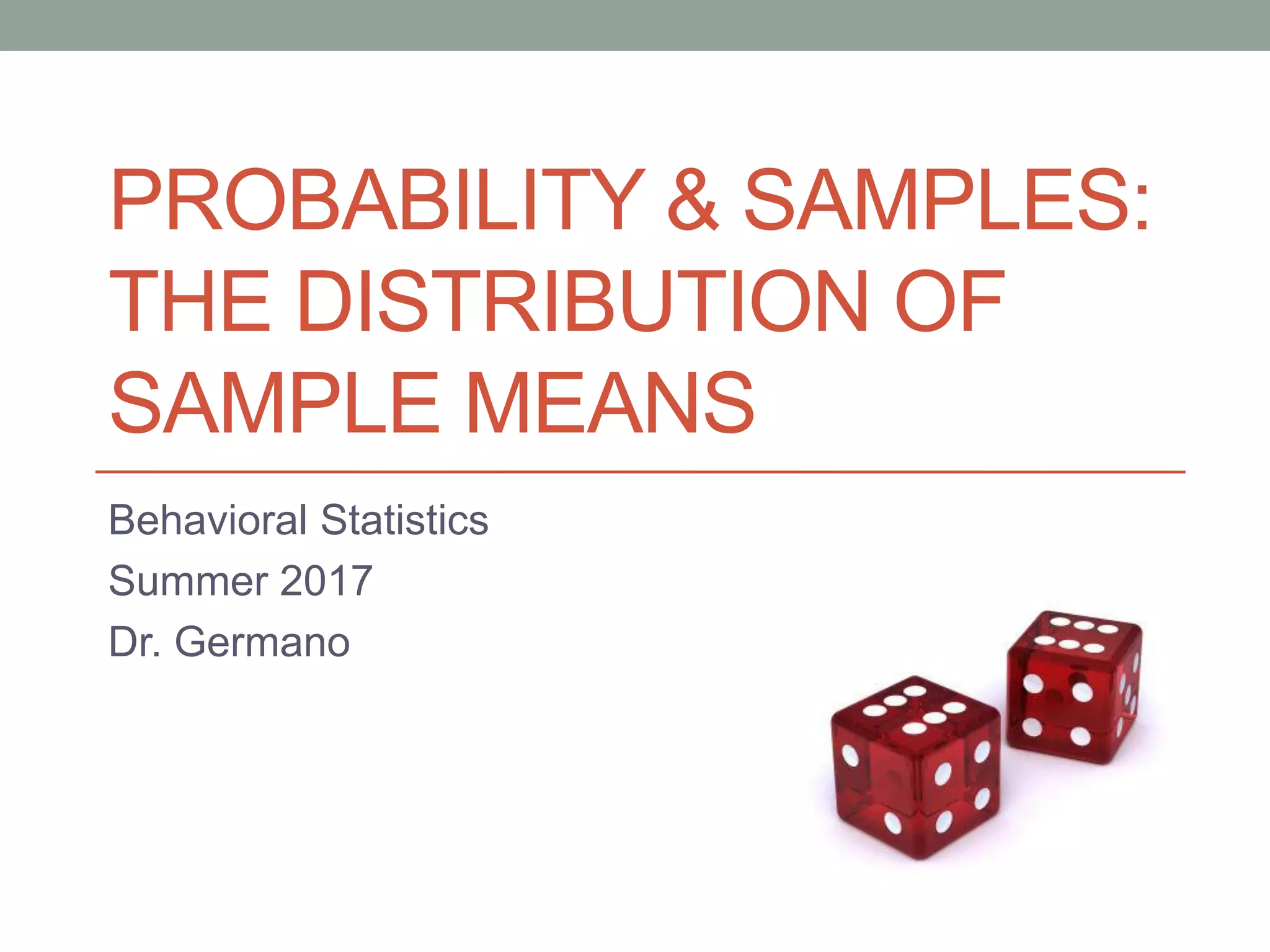
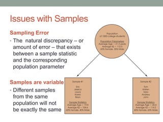
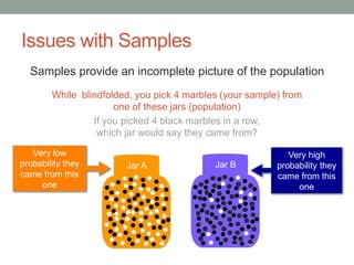
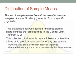
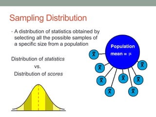
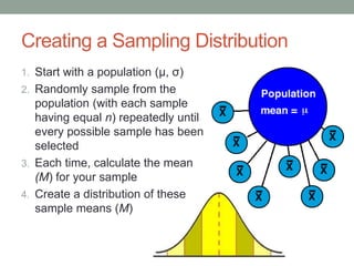
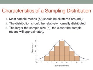
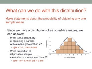
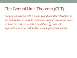
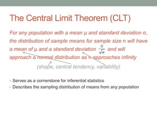
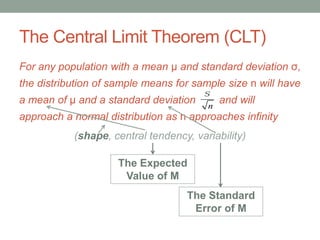
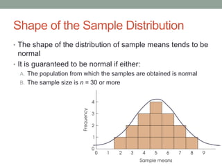
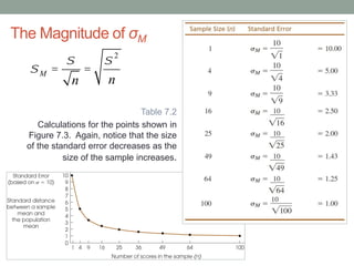
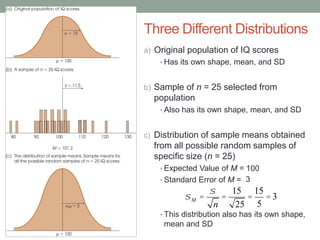
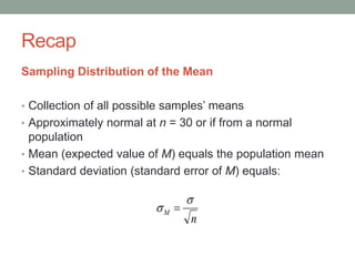
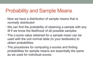
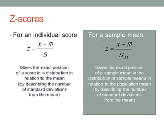
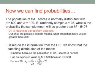
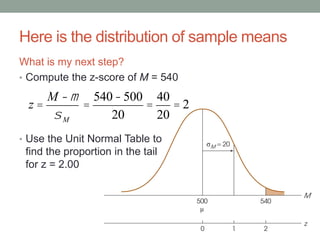
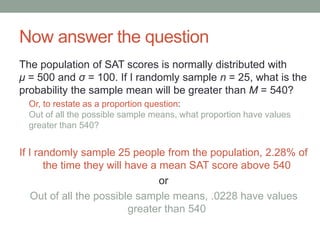
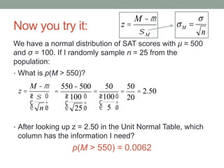
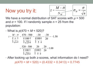
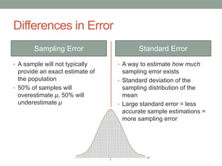
PROBABILITY & SAMPLES:
THE DISTRIBUTION OF
SAMPLE MEANS
Behavioral Statistics
Summer 2017
Dr. Germano
What we’ve
learned so
far…
Thus far, we have been talking about
probabilities for a single event (n = 1)
In Chapter 5…
Z-scores help us
determine a score’s
exact position in a
distribution in terms
of standard
deviations from the
mean
In Chapter 6…
If the variable is
normally distributed,
we can use the z-
score to determine
exact probabilities for
obtaining any
individual score
68.26%
94.46%
99.73%
Samples and Populations
• Typically, samples are much larger than n = 1
• How can we move from considering the probability of a
single score to considering the probability of a group of
scores?
• Find some value that is a representative value of that sample, and
convert that into a z-score to represent the sample.
• What single value could we use to represent a group of
scores?
• The mean (‘typical’/ ‘central’)
Now we can begin to think about the probability of
obtaining a certain sample from the population
(vs. a single score)
Issues with Samples
Sampling Error
• The natural discrepancy – or
amount of error – that exists
between a sample statistic
and the corresponding
population parameter
Samples are variable
• Different samples
from the same
population will not
be exactly the same
Issues with Samples
Samples provide an incomplete picture of the population
While blindfolded, you pick 4 marbles (your sample) from
one of these jars (population)
If you picked 4 black marbles in a row,
which jar would say they came from?
Jar A
Very low
probability they
came from this
one
Jar B
Jar B
Very high
probability they
came from this
one
THE DISTRIBUTION OF
SAMPLE MEANS
Distribution of Sample Means
The set of sample means from all the possible random
samples of a specific size (n) selected from a specific
population
• This distribution has well-defined (and predictable)
characteristics that are specified in the Central Limit
Theorem (CLT)
• This collection of all sample means follows a pattern that
allows us to predict characteristics of any one sample
• Much like the z-score distribution allows us to predict
characteristics of any one score from a normally distributed variable
• A distribution of statistics obtained by
selecting all the possible samples of
a specific size from a population
Distribution of statistics
vs.
Distribution of scores
Sampling Distribution
Creating a Sampling Distribution
1. Start with a population (µ, σ)
2. Randomly sample from the
population (with each sample
having equal n) repeatedly until
every possible sample has been
selected
3. Each time, calculate the mean
(M) for your sample
4. Create a distribution of these
sample means (M)
Example 7.1
Step 1 is to start with a population
• Figure 7.1 is a frequency distribution histogram for a population of 4
scores: 2, 4, 6, 8
Example 7.1
Step 2 is to randomly sample from the population (equal n’s)
until every possible sample has been selected
• Table 7.1 lists all possible samples
of n = 2 scores that can be
obtained from the population
presented in Figure 7.1
• Note that the table lists random
samples.
• This requires sampling with
replacement, so it is possible to
select the same score twice.
Step 3 is to calculate the mean
(M) for each sample
Example 7.1
Step 4 is to create a distribution of these sample means (M)
• Figure 7.2 shows the distribution of 16 sample means
from Table 7.1
Characteristics of a Sampling Distribution
1. Most sample means (M) should be clustered around μ
2. The distribution should be relatively normally distributed
3. The larger the sample size (n), the closer the sample
means will approximate μ
What can we do with this distribution?
Make statements about the probability of obtaining any one
sample mean
• Since we have a distribution of all possible samples, we
can answer:
• What is the probability
of obtaining a sample
with a mean greater than 7?
• p(M > 7) = 1/16 = 0.063
• What proportion of
all possible sample
means have a value less than 5?
• p(M < 5) = 6/16 or 3/8 = 0.375
Is the Sampling Distribution Useful?
YES
• Typically when we conduct research, we deal with very
large populations and it is not realistic to believe we will
be able to measure every possible sample
How is the sampling distribution useful?
• If all sampling distributions of the mean follow a similar
mathematical pattern (the Central Limit Theorem), we will
know how the distribution will behave without actually
creating it.
• Then, we can still make claims about the likelihood of our
one sample considering all possible samples
The Central Limit Theorem (CLT)
For any population with a mean μ and standard deviation σ,
the distribution of sample means for sample size n will have
a mean of μ and a standard deviation and will
approach a normal distribution as n approaches infinity
s
n
The Central Limit Theorem (CLT)
For any population with a mean μ and standard deviation σ,
the distribution of sample means for sample size n will have
a mean of μ and a standard deviation and will
approach a normal distribution as n approaches infinity
(shape, central tendency, variability)
• Serves as a cornerstone for inferential statistics
• Describes the sampling distribution of means from any population
s
n
The Central Limit Theorem (CLT)
For any population with a mean μ and standard deviation σ,
the distribution of sample means for sample size n will have
a mean of μ and a standard deviation and will
approach a normal distribution as n approaches infinity
(shape, central tendency, variability)
s
n
The Expected
Value of M
The Standard
Error of M
Shape of the Sample Distribution
• The shape of the distribution of sample means tends to be
normal
• It is guaranteed to be normal if either:
A. The population from which the samples are obtained is normal
B. The sample size is n = 30 or more
The Expected Value of M
The mean of the distribution of sample means is always
equal to the mean of the population of scores (μ)
• If two (or more) samples are selected from the same
population, the two samples probably will have different
means.
• Although the samples will have different means, you
should expect the sample means to be close to the
population mean
• an unbaised statistic; accurately describes the population mean
• Thus, the average value of all possible sample means will
equal exactly the population parameter
The Standard Error of M (σM)
The standard deviation of the distribution of sample means
• = standard distance between M and μ
• Two general purposes:
1. Describes the distribution of sample means
• A measure of how much difference is expected from one sample to
another
2. Measures how well an individual sample mean represents an
entire distribution
• Provides a measure of how much distance is reasonable to expect
between M and μ
• The magnitude of is determined by:
1. The size of the sample (n), and
2. The standard deviation (σ) of the population
M
M
The Magnitude of σM
1. The influence of n
In general, as n increases, the error between M and μ
decreases
(the inverse is also true: as n decreases, the error increases)
Law of Large Numbers:
the larger the n, the more probable it is
that M will be close to μ
The Magnitude of σM
2. The influence of σ
• Large n = smaller error; small n = larger error
• Consider σ as the “starting point” for standard error
• When n = 1:
• We have one score (X)
• The sample mean: M = X
• Standard error (σM) = standard distance between X and μ
• Therefore, σM = σ
• In the situation with the largest possible standard error, it is equal to
the population standard deviation
The Magnitude of σM
2. The influence of σ (continued)
• What should happen to the standard error as we get
more information (as n increases)?
• It should become smaller in a way that takes into account how
much information we have
The Magnitude of σM
Table 7.2
Calculations for the points shown in
Figure 7.3. Again, notice that the size
of the standard error decreases as the
size of the sample increases.
sM =
s
n
=
s 2
n
Three Different Distributions
a) Original population of IQ scores
• Has its own shape, mean, and SD
b) Sample of n = 25 selected from
population
• Also has its own shape, mean, and SD
c) Distribution of sample means obtained
from all possible random samples of
specific size (n = 25)
• Expected Value of M =
• Standard Error of M =
• This distribution also has its own shape,
mean and SD
sM =
s
n
100
3
=
15
25
=
15
5
= 3
PROBABILITY AND THE
DISTRIBUTION OF SAMPLE
MEANS
Recap
Sampling Distribution of the Mean
• Collection of all possible samples’ means
• Approximately normal at n = 30 or if from a normal
population
• Mean (expected value of M) equals the population mean
• Standard deviation (standard error of M) equals:
n
M

 
Probability and Sample Means
• Now we have a distribution of sample means that is
normally distributed
• We can find the probability of obtaining a sample with any
M if we know the likelihood of all possible samples
• The z-score value obtained for a sample mean can be
used with the unit normal table (in your textbooks) to
obtain probabilities
• The procedures for computing z-scores and finding
probabilities for sample means are essentially the same
as we used for individual scores
Z-scores
• For an individual score
Gives the exact position
of a score in a distribution in
relation to the mean
(by describing the number
of standard deviations
from the mean)
• For a sample mean
Gives the exact position
of a sample mean in the
distribution of sample means in
relation to the population mean
(by describing the number
of standard deviations
from the mean)
z =
x -m
s
z =
x -m
sM
Now we can find probabilities…
The population of SAT scores is normally distributed with
μ = 500 and σ = 100. If I randomly sample n = 25, what is the
probability the sample mean will be greater than M = 540?
Or, to restate as a proportion question:
Out of all the possible sample means, what proportion have values
greater than 540?
• Based on the information from the CLT, we know that the
sampling distribution of the mean:
• Is normal because the population of SAT scores is normal
• Has an expected value of M = 500 because μ = 500
• For n = 20, sM =
s
n
=
100
25
= 20
Here is the distribution of sample means
What is my next step?
• Compute the z-score of M = 540
• Use the Unit Normal Table to
find the proportion in the tail
for z = 2.00
z =
M -m
sM
=
540-500
20
=
40
20
= 2
Now answer the question
The population of SAT scores is normally distributed with
μ = 500 and σ = 100. If I randomly sample n = 25, what is the
probability the sample mean will be greater than M = 540?
Or, to restate as a proportion question:
Out of all the possible sample means, what proportion have values
greater than 540?
If I randomly sample 25 people from the population, 2.28% of
the time they will have a mean SAT score above 540
or
Out of all the possible sample means, .0228 have values
greater than 540
Now you try it:
• What is p(M > 550)?
• After looking up z = 2.50 in the Unit Normal Table, which
column has the information I need?
p(M > 550) = 0.0062
We have a normal distribution of SAT scores with μ = 500
and σ = 100. If I randomly sample n = 25 from the
population:
z =
M -m
s
n
æ
è
ç
ö
ø
÷
z =
M -m
sM n
M

 
=
550-500
100
25
æ
è
ç
ö
ø
÷
=
50
100
5
æ
è
ç
ö
ø
÷
=
50
20
= 2.50
Now you try it:
• What is p(470 < M < 520)?
• After looking up both z-scores, what information do I need?
p(470 < M < 520) = (0.4332 + 0.3413) = 0.7745
We have a normal distribution of SAT scores with μ = 500
and σ = 100. If I randomly sample n = 25 from the
population:
z =
M -m
s
n
æ
è
ç
ö
ø
÷
z =
M -m
sM n
M

 
=
470-500
100
25
æ
è
ç
ö
ø
÷
=
-30
100
5
æ
è
ç
ö
ø
÷
=
-30
20
= -1.50
=
520-500
100
25
æ
è
ç
ö
ø
÷
=
20
100
5
æ
è
ç
ö
ø
÷
=
20
20
=1.00
MORE ABOUT STANDARD
ERROR
Differences in Error
Sampling Error
• A sample will not typically
provide an exact estimate of
the population
• 50% of samples will
overestimate μ, 50% will
underestimate μ
Standard Error
• A way to estimate how much
sampling error exists
• Standard deviation of the
sampling distribution of the
mean
• Large standard error = less
accurate sample estimations =
more sampling error
LOOKING AHEAD TO
INFERENTIAL STATISTICS
Looking ahead
• Natural differences exist between statistics and
parameters
• Samples are not perfect representatives and there will
always be some error
• Sampling error of M
• There will always be some amount of uncertainty when
trying to generalize to a population from a sample
How can we use these concepts to help
draw inferences?
• We have a population
• All students in the class
• We know how this population performs
• Population μ and σ on a typical test
• We can sample from this population
• Randomly sample n = 5 students
• Give them some treatment
• Special study sessions
• And see if they have a mean noticeably different than the
population
• If the sample scores noticeably higher than typical, we have
evidence that these study sessions ‘work’
The Point for Inferential Statistics
If I know the distribution of all possible means… then I can
make judgments about whether an event is unlikely or
atypical
• Is an event likely to occur by chance given how all
possible events occur?
• Or is an event unlikely and thus attributed to some other
factor than chance?
• (i.e., treatment, intervention, etc.)

Probability & Samples

  • 1.
    PROBABILITY & SAMPLES: THEDISTRIBUTION OF SAMPLE MEANS Behavioral Statistics Summer 2017 Dr. Germano
  • 2.
    What we’ve learned so far… Thusfar, we have been talking about probabilities for a single event (n = 1) In Chapter 5… Z-scores help us determine a score’s exact position in a distribution in terms of standard deviations from the mean In Chapter 6… If the variable is normally distributed, we can use the z- score to determine exact probabilities for obtaining any individual score 68.26% 94.46% 99.73%
  • 3.
    Samples and Populations •Typically, samples are much larger than n = 1 • How can we move from considering the probability of a single score to considering the probability of a group of scores? • Find some value that is a representative value of that sample, and convert that into a z-score to represent the sample. • What single value could we use to represent a group of scores? • The mean (‘typical’/ ‘central’) Now we can begin to think about the probability of obtaining a certain sample from the population (vs. a single score)
  • 4.
    Issues with Samples SamplingError • The natural discrepancy – or amount of error – that exists between a sample statistic and the corresponding population parameter Samples are variable • Different samples from the same population will not be exactly the same
  • 5.
    Issues with Samples Samplesprovide an incomplete picture of the population While blindfolded, you pick 4 marbles (your sample) from one of these jars (population) If you picked 4 black marbles in a row, which jar would say they came from? Jar A Very low probability they came from this one Jar B Jar B Very high probability they came from this one
  • 6.
  • 7.
    Distribution of SampleMeans The set of sample means from all the possible random samples of a specific size (n) selected from a specific population • This distribution has well-defined (and predictable) characteristics that are specified in the Central Limit Theorem (CLT) • This collection of all sample means follows a pattern that allows us to predict characteristics of any one sample • Much like the z-score distribution allows us to predict characteristics of any one score from a normally distributed variable
  • 8.
    • A distributionof statistics obtained by selecting all the possible samples of a specific size from a population Distribution of statistics vs. Distribution of scores Sampling Distribution
  • 9.
    Creating a SamplingDistribution 1. Start with a population (µ, σ) 2. Randomly sample from the population (with each sample having equal n) repeatedly until every possible sample has been selected 3. Each time, calculate the mean (M) for your sample 4. Create a distribution of these sample means (M)
  • 10.
    Example 7.1 Step 1is to start with a population • Figure 7.1 is a frequency distribution histogram for a population of 4 scores: 2, 4, 6, 8
  • 11.
    Example 7.1 Step 2is to randomly sample from the population (equal n’s) until every possible sample has been selected • Table 7.1 lists all possible samples of n = 2 scores that can be obtained from the population presented in Figure 7.1 • Note that the table lists random samples. • This requires sampling with replacement, so it is possible to select the same score twice. Step 3 is to calculate the mean (M) for each sample
  • 12.
    Example 7.1 Step 4is to create a distribution of these sample means (M) • Figure 7.2 shows the distribution of 16 sample means from Table 7.1
  • 13.
    Characteristics of aSampling Distribution 1. Most sample means (M) should be clustered around μ 2. The distribution should be relatively normally distributed 3. The larger the sample size (n), the closer the sample means will approximate μ
  • 14.
    What can wedo with this distribution? Make statements about the probability of obtaining any one sample mean • Since we have a distribution of all possible samples, we can answer: • What is the probability of obtaining a sample with a mean greater than 7? • p(M > 7) = 1/16 = 0.063 • What proportion of all possible sample means have a value less than 5? • p(M < 5) = 6/16 or 3/8 = 0.375
  • 15.
    Is the SamplingDistribution Useful? YES • Typically when we conduct research, we deal with very large populations and it is not realistic to believe we will be able to measure every possible sample How is the sampling distribution useful? • If all sampling distributions of the mean follow a similar mathematical pattern (the Central Limit Theorem), we will know how the distribution will behave without actually creating it. • Then, we can still make claims about the likelihood of our one sample considering all possible samples
  • 16.
    The Central LimitTheorem (CLT) For any population with a mean μ and standard deviation σ, the distribution of sample means for sample size n will have a mean of μ and a standard deviation and will approach a normal distribution as n approaches infinity s n
  • 17.
    The Central LimitTheorem (CLT) For any population with a mean μ and standard deviation σ, the distribution of sample means for sample size n will have a mean of μ and a standard deviation and will approach a normal distribution as n approaches infinity (shape, central tendency, variability) • Serves as a cornerstone for inferential statistics • Describes the sampling distribution of means from any population s n
  • 18.
    The Central LimitTheorem (CLT) For any population with a mean μ and standard deviation σ, the distribution of sample means for sample size n will have a mean of μ and a standard deviation and will approach a normal distribution as n approaches infinity (shape, central tendency, variability) s n The Expected Value of M The Standard Error of M
  • 19.
    Shape of theSample Distribution • The shape of the distribution of sample means tends to be normal • It is guaranteed to be normal if either: A. The population from which the samples are obtained is normal B. The sample size is n = 30 or more
  • 20.
    The Expected Valueof M The mean of the distribution of sample means is always equal to the mean of the population of scores (μ) • If two (or more) samples are selected from the same population, the two samples probably will have different means. • Although the samples will have different means, you should expect the sample means to be close to the population mean • an unbaised statistic; accurately describes the population mean • Thus, the average value of all possible sample means will equal exactly the population parameter
  • 21.
    The Standard Errorof M (σM) The standard deviation of the distribution of sample means • = standard distance between M and μ • Two general purposes: 1. Describes the distribution of sample means • A measure of how much difference is expected from one sample to another 2. Measures how well an individual sample mean represents an entire distribution • Provides a measure of how much distance is reasonable to expect between M and μ • The magnitude of is determined by: 1. The size of the sample (n), and 2. The standard deviation (σ) of the population M M
  • 22.
    The Magnitude ofσM 1. The influence of n In general, as n increases, the error between M and μ decreases (the inverse is also true: as n decreases, the error increases) Law of Large Numbers: the larger the n, the more probable it is that M will be close to μ
  • 23.
    The Magnitude ofσM 2. The influence of σ • Large n = smaller error; small n = larger error • Consider σ as the “starting point” for standard error • When n = 1: • We have one score (X) • The sample mean: M = X • Standard error (σM) = standard distance between X and μ • Therefore, σM = σ • In the situation with the largest possible standard error, it is equal to the population standard deviation
  • 24.
    The Magnitude ofσM 2. The influence of σ (continued) • What should happen to the standard error as we get more information (as n increases)? • It should become smaller in a way that takes into account how much information we have
  • 25.
    The Magnitude ofσM Table 7.2 Calculations for the points shown in Figure 7.3. Again, notice that the size of the standard error decreases as the size of the sample increases. sM = s n = s 2 n
  • 26.
    Three Different Distributions a)Original population of IQ scores • Has its own shape, mean, and SD b) Sample of n = 25 selected from population • Also has its own shape, mean, and SD c) Distribution of sample means obtained from all possible random samples of specific size (n = 25) • Expected Value of M = • Standard Error of M = • This distribution also has its own shape, mean and SD sM = s n 100 3 = 15 25 = 15 5 = 3
  • 27.
  • 28.
    Recap Sampling Distribution ofthe Mean • Collection of all possible samples’ means • Approximately normal at n = 30 or if from a normal population • Mean (expected value of M) equals the population mean • Standard deviation (standard error of M) equals: n M   
  • 29.
    Probability and SampleMeans • Now we have a distribution of sample means that is normally distributed • We can find the probability of obtaining a sample with any M if we know the likelihood of all possible samples • The z-score value obtained for a sample mean can be used with the unit normal table (in your textbooks) to obtain probabilities • The procedures for computing z-scores and finding probabilities for sample means are essentially the same as we used for individual scores
  • 30.
    Z-scores • For anindividual score Gives the exact position of a score in a distribution in relation to the mean (by describing the number of standard deviations from the mean) • For a sample mean Gives the exact position of a sample mean in the distribution of sample means in relation to the population mean (by describing the number of standard deviations from the mean) z = x -m s z = x -m sM
  • 31.
    Now we canfind probabilities… The population of SAT scores is normally distributed with μ = 500 and σ = 100. If I randomly sample n = 25, what is the probability the sample mean will be greater than M = 540? Or, to restate as a proportion question: Out of all the possible sample means, what proportion have values greater than 540? • Based on the information from the CLT, we know that the sampling distribution of the mean: • Is normal because the population of SAT scores is normal • Has an expected value of M = 500 because μ = 500 • For n = 20, sM = s n = 100 25 = 20
  • 32.
    Here is thedistribution of sample means What is my next step? • Compute the z-score of M = 540 • Use the Unit Normal Table to find the proportion in the tail for z = 2.00 z = M -m sM = 540-500 20 = 40 20 = 2
  • 33.
    Now answer thequestion The population of SAT scores is normally distributed with μ = 500 and σ = 100. If I randomly sample n = 25, what is the probability the sample mean will be greater than M = 540? Or, to restate as a proportion question: Out of all the possible sample means, what proportion have values greater than 540? If I randomly sample 25 people from the population, 2.28% of the time they will have a mean SAT score above 540 or Out of all the possible sample means, .0228 have values greater than 540
  • 34.
    Now you tryit: • What is p(M > 550)? • After looking up z = 2.50 in the Unit Normal Table, which column has the information I need? p(M > 550) = 0.0062 We have a normal distribution of SAT scores with μ = 500 and σ = 100. If I randomly sample n = 25 from the population: z = M -m s n æ è ç ö ø ÷ z = M -m sM n M    = 550-500 100 25 æ è ç ö ø ÷ = 50 100 5 æ è ç ö ø ÷ = 50 20 = 2.50
  • 35.
    Now you tryit: • What is p(470 < M < 520)? • After looking up both z-scores, what information do I need? p(470 < M < 520) = (0.4332 + 0.3413) = 0.7745 We have a normal distribution of SAT scores with μ = 500 and σ = 100. If I randomly sample n = 25 from the population: z = M -m s n æ è ç ö ø ÷ z = M -m sM n M    = 470-500 100 25 æ è ç ö ø ÷ = -30 100 5 æ è ç ö ø ÷ = -30 20 = -1.50 = 520-500 100 25 æ è ç ö ø ÷ = 20 100 5 æ è ç ö ø ÷ = 20 20 =1.00
  • 36.
  • 37.
    Differences in Error SamplingError • A sample will not typically provide an exact estimate of the population • 50% of samples will overestimate μ, 50% will underestimate μ Standard Error • A way to estimate how much sampling error exists • Standard deviation of the sampling distribution of the mean • Large standard error = less accurate sample estimations = more sampling error
  • 38.
  • 39.
    Looking ahead • Naturaldifferences exist between statistics and parameters • Samples are not perfect representatives and there will always be some error • Sampling error of M • There will always be some amount of uncertainty when trying to generalize to a population from a sample
  • 40.
    How can weuse these concepts to help draw inferences? • We have a population • All students in the class • We know how this population performs • Population μ and σ on a typical test • We can sample from this population • Randomly sample n = 5 students • Give them some treatment • Special study sessions • And see if they have a mean noticeably different than the population • If the sample scores noticeably higher than typical, we have evidence that these study sessions ‘work’
  • 41.
    The Point forInferential Statistics If I know the distribution of all possible means… then I can make judgments about whether an event is unlikely or atypical • Is an event likely to occur by chance given how all possible events occur? • Or is an event unlikely and thus attributed to some other factor than chance? • (i.e., treatment, intervention, etc.)