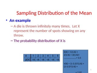
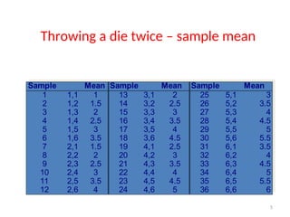
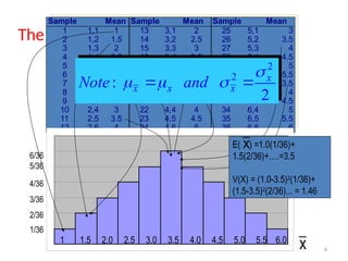
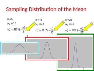
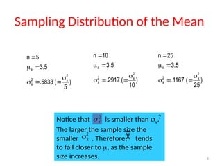
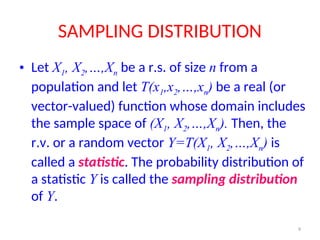
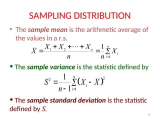
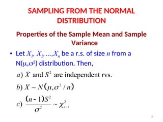
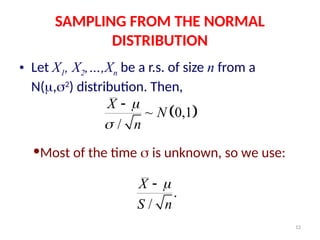
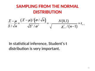
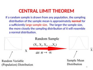
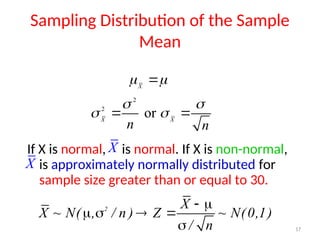
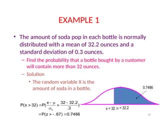
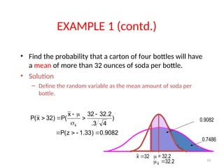
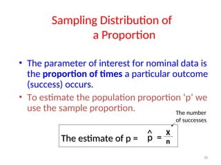
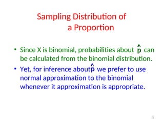
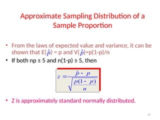
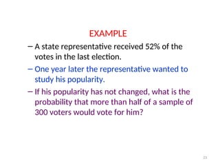
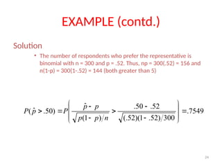
SAMPLING DISTRIBUTION
2
Introduction
• In real life calculating parameters of populations is
usually impossible because populations are very
large.
• Rather than investigating the whole population,
we take a sample, calculate a statistic related to
the parameter of interest, and make an inference.
• The sampling distribution of the statistic is the
tool that tells us how close is the statistic to the
parameter.
3
Sampling Distribution of the Mean
• An example
– A die is thrown infinitely many times. Let X
represent the number of spots showing on any
throw.
– The probability distribution of X is
x 1 2 3 4 5 6
p(x) 1/6 1/6 1/6 1/6 1/6 1/6
E(X) = 1(1/6) +
2(1/6) + 3(1/6)+
………………….= 3.5
V(X) = (1-3.5)2
(1/6) +
(2-3.5)2
(1/6) +
4
• Suppose we want to estimate  from
the mean of a sample of size n = 2.
• What is the distribution of ?
X
Throwing a die twice – sample mean
X
5
Sample Mean Sample Mean Sample Mean
1 1,1 1 13 3,1 2 25 5,1 3
2 1,2 1.5 14 3,2 2.5 26 5,2 3.5
3 1,3 2 15 3,3 3 27 5,3 4
4 1,4 2.5 16 3,4 3.5 28 5,4 4.5
5 1,5 3 17 3,5 4 29 5,5 5
6 1,6 3.5 18 3,6 4.5 30 5,6 5.5
7 2,1 1.5 19 4,1 2.5 31 6,1 3.5
8 2,2 2 20 4,2 3 32 6,2 4
9 2,3 2.5 21 4,3 3.5 33 6,3 4.5
10 2,4 3 22 4,4 4 34 6,4 5
11 2,5 3.5 23 4,5 4.5 35 6,5 5.5
12 2,6 4 24 4,6 5 36 6,6 6
Throwing a die twice – sample mean
6
X
The distribution of when n = 2
Sample Mean Sample Mean Sample Mean
1 1,1 1 13 3,1 2 25 5,1 3
2 1,2 1.5 14 3,2 2.5 26 5,2 3.5
3 1,3 2 15 3,3 3 27 5,3 4
4 1,4 2.5 16 3,4 3.5 28 5,4 4.5
5 1,5 3 17 3,5 4 29 5,5 5
6 1,6 3.5 18 3,6 4.5 30 5,6 5.5
7 2,1 1.5 19 4,1 2.5 31 6,1 3.5
8 2,2 2 20 4,2 3 32 6,2 4
9 2,3 2.5 21 4,3 3.5 33 6,3 4.5
10 2,4 3 22 4,4 4 34 6,4 5
11 2,5 3.5 23 4,5 4.5 35 6,5 5.5
12 2,6 4 24 4,6 5 36 6,6 6
1 1.5 2.0 2.5 3.0 3.5 4.0 4.5 5.0 5.5 6.0
6/36
5/36
4/36
3/36
2/36
1/36
x
E( ) =1.0(1/36)+
1.5(2/36)+….=3.5
V(X) = (1.0-3.5)2
(1/36)+
(1.5-3.5)2
(2/36)... = 1.46
x
2
2
:
2
x
x x x
Note and

  
 
7
6
)
5
(
5833
.
5
.
3
5
n
2
x
2
x
x







)
10
(
2917
.
5
.
3
10
n
2
x
2
x
x







)
25
(
1167
.
5
.
3
25
n
2
x
2
x
x







Sampling Distribution of the Mean
8
Sampling Distribution of the Mean
)
5
(
5833
.
5
.
3
5
n
2
x
2
x
x







)
10
(
2917
.
5
.
3
10
n
2
x
2
x
x







)
25
(
1167
.
5
.
3
25
n
2
x
2
x
x







Notice that is smaller than .
The larger the sample size the
smaller . Therefore, tends
to fall closer to , as the sample
size increases.
2
x

x
2
x

Notice that is smaller than x.
The larger the sample size the
smaller . Therefore, tends
to fall closer to , as the sample
size increases.
2
x

x
2
x

2
9
SAMPLING DISTRIBUTION
• Let X1, X2,…,Xn be a r.s. of size n from a
population and let T(x1,x2,…,xn) be a real (or
vector-valued) function whose domain includes
the sample space of (X1, X2,…,Xn). Then, the
r.v. or a random vector Y=T(X1, X2,…,Xn) is
called a statistic. The probability distribution of
a statistic Y is called the sampling distribution
of Y.
10
SAMPLING DISTRIBUTION
• The sample mean is the arithmetic average of
the values in a r.s.
1 2
1
1 n
n
i
i
X X X
X X
n n 
  
  

• The sample variance is the statistic defined by
 
2
2
1
1
1
n
i
i
S X X
n 
 


• The sample standard deviation is the statistic
defined by S.
11
SAMPLING FROM THE NORMAL
DISTRIBUTION
Properties of the Sample Mean and Sample
Variance
• Let X1, X2,…,Xn be a r.s. of size n from a
N(,2
) distribution. Then,
2
) and are independent rvs.
a X S
 
2
) ~ , /
b X N n
 
  2
2
1
2
1
) ~ n
n S
c 
 

12
SAMPLING FROM THE NORMAL
DISTRIBUTION
• Let X1, X2,…,Xn be a r.s. of size n from a
N(,2
) distribution. Then,
 
~ 0,1
/
X
N
n



•Most of the time  is unknown, so we use:
.
/
X
S n


13
SAMPLING FROM THE NORMAL
DISTRIBUTION
In statistical inference, Student’s t
distribution is very important.
14
SAMPLING FROM THE NORMAL
DISTRIBUTION
• Let X1, X2,…,Xn be a r.s. of size n from a
N(X,X
2
) distribution and let Y1,Y2,…,Ym
be a r.s. of size m from an independent
N(Y,Y
2
).
• If we are interested in comparing the
variability of the populations, one
quantity of interest would be the ratio
2 2 2 2
/ /
X Y X Y
S S
  
15
SAMPLING FROM THE NORMAL
DISTRIBUTION
• The F distribution allows us to compare these
quantities by giving the distribution of
2 2 2 2
1, 1
2 2 2 2
/ /
~
/ /
X Y X X
n m
X Y Y Y
S S S
F
S

    

• If X~Fp,q, then 1/X~Fq,p.
• If X~tq, then X2
~F1,q.
16
CENTRAL LIMIT THEOREM
If a random sample is drawn from any population, the sampling
distribution of the sample mean is approximately normal for
a sufficiently large sample size. The larger the sample size,
the more closely the sampling distribution of X will resemble
a normal distribution.
Random Sample
(X1, X2, X3, …,Xn)
Sample Mean
Distribution
X
X
Random Variable
(Population) Distribution
as n  
17
Sampling Distribution of the Sample
Mean
If X is normal, is normal. If X is non-normal,
is approximately normally distributed for
sample size greater than or equal to 30.
X
 

2
2
or
X X
n n
 
 
 
X
X
2 X
X ~ N( , / n ) Z ~ N(0,1)
/ n
 
   

18
• The amount of soda pop in each bottle is normally
distributed with a mean of 32.2 ounces and a
standard deviation of 0.3 ounces.
– Find the probability that a bottle bought by a customer
will contain more than 32 ounces.
– Solution
• The random variable X is the
amount of soda in a bottle.
 = 32.2
0.7486
x = 32
7486
.
0
)
67
.
z
(
P
)
3
.
2
.
32
32
x
(
P
)
32
x
(
P
x











EXAMPLE 1
19
 = 32.2
0.7486
x = 32
• Find the probability that a carton of four bottles will have
a mean of more than 32 ounces of soda per bottle.
• Solution
– Define the random variable as the mean amount of soda per
bottle.
9082
.
0
)
33
.
1
z
(
P
)
4
3
.
2
.
32
32
x
(
P
)
32
x
(
P
x











32
x 
0.9082
2
.
32
x 

EXAMPLE 1 (contd.)
20
The estimate of p =
The estimate of p =
• The parameter of interest for nominal data is
the proportion of times a particular outcome
(success) occurs.
• To estimate the population proportion ‘p’ we
use the sample proportion.
Sampling Distribution of
a Proportion
p
p
^
^ =
=
X
X
n
n
The number
of successes
21
• Since X is binomial, probabilities about can
be calculated from the binomial distribution.
• Yet, for inference about we prefer to use
normal approximation to the binomial
whenever it approximation is appropriate.
p
p
^
^
Sampling Distribution of
a Proportion
p
p
^
^
22
Approximate Sampling Distribution of a
Sample Proportion
• From the laws of expected value and variance, it can be
shown that E( ) = p and V( )=p(1-p)/n
• If both np ≥ 5 and n(1-p) ≥ 5, then
• Z is approximately standard normally distributed.
ˆ
(1 )
p p
z
p p
n



p̂ p̂
23
EXAMPLE
– A state representative received 52% of the
votes in the last election.
– One year later the representative wanted to
study his popularity.
– If his popularity has not changed, what is the
probability that more than half of a sample of
300 voters would vote for him?
24
EXAMPLE (contd.)
Solution
• The number of respondents who prefer the representative is
binomial with n = 300 and p = .52. Thus, np = 300(.52) = 156 and
n(1-p) = 300(1-.52) = 144 (both greater than 5)
7549
.
300
)
52
.
1
)(
52
(.
52
.
50
.
)
1
(
ˆ
)
50
.
ˆ
( 















n
p
p
p
p
P
p
P

RANDOM VARIABLE SAMPLING DISTRIBUTION.ppt

  • 1.
  • 2.
    2 Introduction • In reallife calculating parameters of populations is usually impossible because populations are very large. • Rather than investigating the whole population, we take a sample, calculate a statistic related to the parameter of interest, and make an inference. • The sampling distribution of the statistic is the tool that tells us how close is the statistic to the parameter.
  • 3.
    3 Sampling Distribution ofthe Mean • An example – A die is thrown infinitely many times. Let X represent the number of spots showing on any throw. – The probability distribution of X is x 1 2 3 4 5 6 p(x) 1/6 1/6 1/6 1/6 1/6 1/6 E(X) = 1(1/6) + 2(1/6) + 3(1/6)+ ………………….= 3.5 V(X) = (1-3.5)2 (1/6) + (2-3.5)2 (1/6) +
  • 4.
    4 • Suppose wewant to estimate  from the mean of a sample of size n = 2. • What is the distribution of ? X Throwing a die twice – sample mean X
  • 5.
    5 Sample Mean SampleMean Sample Mean 1 1,1 1 13 3,1 2 25 5,1 3 2 1,2 1.5 14 3,2 2.5 26 5,2 3.5 3 1,3 2 15 3,3 3 27 5,3 4 4 1,4 2.5 16 3,4 3.5 28 5,4 4.5 5 1,5 3 17 3,5 4 29 5,5 5 6 1,6 3.5 18 3,6 4.5 30 5,6 5.5 7 2,1 1.5 19 4,1 2.5 31 6,1 3.5 8 2,2 2 20 4,2 3 32 6,2 4 9 2,3 2.5 21 4,3 3.5 33 6,3 4.5 10 2,4 3 22 4,4 4 34 6,4 5 11 2,5 3.5 23 4,5 4.5 35 6,5 5.5 12 2,6 4 24 4,6 5 36 6,6 6 Throwing a die twice – sample mean
  • 6.
    6 X The distribution ofwhen n = 2 Sample Mean Sample Mean Sample Mean 1 1,1 1 13 3,1 2 25 5,1 3 2 1,2 1.5 14 3,2 2.5 26 5,2 3.5 3 1,3 2 15 3,3 3 27 5,3 4 4 1,4 2.5 16 3,4 3.5 28 5,4 4.5 5 1,5 3 17 3,5 4 29 5,5 5 6 1,6 3.5 18 3,6 4.5 30 5,6 5.5 7 2,1 1.5 19 4,1 2.5 31 6,1 3.5 8 2,2 2 20 4,2 3 32 6,2 4 9 2,3 2.5 21 4,3 3.5 33 6,3 4.5 10 2,4 3 22 4,4 4 34 6,4 5 11 2,5 3.5 23 4,5 4.5 35 6,5 5.5 12 2,6 4 24 4,6 5 36 6,6 6 1 1.5 2.0 2.5 3.0 3.5 4.0 4.5 5.0 5.5 6.0 6/36 5/36 4/36 3/36 2/36 1/36 x E( ) =1.0(1/36)+ 1.5(2/36)+….=3.5 V(X) = (1.0-3.5)2 (1/36)+ (1.5-3.5)2 (2/36)... = 1.46 x 2 2 : 2 x x x x Note and      
  • 7.
  • 8.
    8 Sampling Distribution ofthe Mean ) 5 ( 5833 . 5 . 3 5 n 2 x 2 x x        ) 10 ( 2917 . 5 . 3 10 n 2 x 2 x x        ) 25 ( 1167 . 5 . 3 25 n 2 x 2 x x        Notice that is smaller than . The larger the sample size the smaller . Therefore, tends to fall closer to , as the sample size increases. 2 x  x 2 x  Notice that is smaller than x. The larger the sample size the smaller . Therefore, tends to fall closer to , as the sample size increases. 2 x  x 2 x  2
  • 9.
    9 SAMPLING DISTRIBUTION • LetX1, X2,…,Xn be a r.s. of size n from a population and let T(x1,x2,…,xn) be a real (or vector-valued) function whose domain includes the sample space of (X1, X2,…,Xn). Then, the r.v. or a random vector Y=T(X1, X2,…,Xn) is called a statistic. The probability distribution of a statistic Y is called the sampling distribution of Y.
  • 10.
    10 SAMPLING DISTRIBUTION • Thesample mean is the arithmetic average of the values in a r.s. 1 2 1 1 n n i i X X X X X n n         • The sample variance is the statistic defined by   2 2 1 1 1 n i i S X X n      • The sample standard deviation is the statistic defined by S.
  • 11.
    11 SAMPLING FROM THENORMAL DISTRIBUTION Properties of the Sample Mean and Sample Variance • Let X1, X2,…,Xn be a r.s. of size n from a N(,2 ) distribution. Then, 2 ) and are independent rvs. a X S   2 ) ~ , / b X N n     2 2 1 2 1 ) ~ n n S c    
  • 12.
    12 SAMPLING FROM THENORMAL DISTRIBUTION • Let X1, X2,…,Xn be a r.s. of size n from a N(,2 ) distribution. Then,   ~ 0,1 / X N n    •Most of the time  is unknown, so we use: . / X S n  
  • 13.
    13 SAMPLING FROM THENORMAL DISTRIBUTION In statistical inference, Student’s t distribution is very important.
  • 14.
    14 SAMPLING FROM THENORMAL DISTRIBUTION • Let X1, X2,…,Xn be a r.s. of size n from a N(X,X 2 ) distribution and let Y1,Y2,…,Ym be a r.s. of size m from an independent N(Y,Y 2 ). • If we are interested in comparing the variability of the populations, one quantity of interest would be the ratio 2 2 2 2 / / X Y X Y S S   
  • 15.
    15 SAMPLING FROM THENORMAL DISTRIBUTION • The F distribution allows us to compare these quantities by giving the distribution of 2 2 2 2 1, 1 2 2 2 2 / / ~ / / X Y X X n m X Y Y Y S S S F S        • If X~Fp,q, then 1/X~Fq,p. • If X~tq, then X2 ~F1,q.
  • 16.
    16 CENTRAL LIMIT THEOREM Ifa random sample is drawn from any population, the sampling distribution of the sample mean is approximately normal for a sufficiently large sample size. The larger the sample size, the more closely the sampling distribution of X will resemble a normal distribution. Random Sample (X1, X2, X3, …,Xn) Sample Mean Distribution X X Random Variable (Population) Distribution as n  
  • 17.
    17 Sampling Distribution ofthe Sample Mean If X is normal, is normal. If X is non-normal, is approximately normally distributed for sample size greater than or equal to 30. X    2 2 or X X n n       X X 2 X X ~ N( , / n ) Z ~ N(0,1) / n       
  • 18.
    18 • The amountof soda pop in each bottle is normally distributed with a mean of 32.2 ounces and a standard deviation of 0.3 ounces. – Find the probability that a bottle bought by a customer will contain more than 32 ounces. – Solution • The random variable X is the amount of soda in a bottle.  = 32.2 0.7486 x = 32 7486 . 0 ) 67 . z ( P ) 3 . 2 . 32 32 x ( P ) 32 x ( P x            EXAMPLE 1
  • 19.
    19  = 32.2 0.7486 x= 32 • Find the probability that a carton of four bottles will have a mean of more than 32 ounces of soda per bottle. • Solution – Define the random variable as the mean amount of soda per bottle. 9082 . 0 ) 33 . 1 z ( P ) 4 3 . 2 . 32 32 x ( P ) 32 x ( P x            32 x  0.9082 2 . 32 x   EXAMPLE 1 (contd.)
  • 20.
    20 The estimate ofp = The estimate of p = • The parameter of interest for nominal data is the proportion of times a particular outcome (success) occurs. • To estimate the population proportion ‘p’ we use the sample proportion. Sampling Distribution of a Proportion p p ^ ^ = = X X n n The number of successes
  • 21.
    21 • Since Xis binomial, probabilities about can be calculated from the binomial distribution. • Yet, for inference about we prefer to use normal approximation to the binomial whenever it approximation is appropriate. p p ^ ^ Sampling Distribution of a Proportion p p ^ ^
  • 22.
    22 Approximate Sampling Distributionof a Sample Proportion • From the laws of expected value and variance, it can be shown that E( ) = p and V( )=p(1-p)/n • If both np ≥ 5 and n(1-p) ≥ 5, then • Z is approximately standard normally distributed. ˆ (1 ) p p z p p n    p̂ p̂
  • 23.
    23 EXAMPLE – A staterepresentative received 52% of the votes in the last election. – One year later the representative wanted to study his popularity. – If his popularity has not changed, what is the probability that more than half of a sample of 300 voters would vote for him?
  • 24.
    24 EXAMPLE (contd.) Solution • Thenumber of respondents who prefer the representative is binomial with n = 300 and p = .52. Thus, np = 300(.52) = 156 and n(1-p) = 300(1-.52) = 144 (both greater than 5) 7549 . 300 ) 52 . 1 )( 52 (. 52 . 50 . ) 1 ( ˆ ) 50 . ˆ (                 n p p p p P p P