Central Limit Theorem
Presented By
Vijeesh
S1-MBA (PT)
Introduction
 The Central Limit Theorem describes
the relationship between the sampling
distribution of sample means and the
population that the samples are taken
from.
Normal Populations
 Important Fact:
 If the population is normally distributed,
then the sampling distribution of x is
normally distributed for any sample size n.
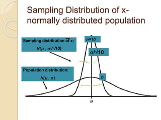
Sampling Distribution of x-
normally distributed population
n=10
/10

Population distribution:
N( , )
Sampling distribution of x:
N( ,  /10)
Non-normal Populations
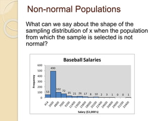
What can we say about the shape of the
sampling distribution of x when the population
from which the sample is selected is not
normal?
53
490
102
72
35 21 26 17 8 10 2 3 1 0 0 1
0
100
200
300
400
500
600
Frequency
Salary ($1,000's)
Baseball Salaries
The Central Limit Theorem
If a random sample of n observations is selected
from a population (any population), then when n is
sufficiently large, the sampling distribution of x will
be approximately normal.
(The larger the sample size, the better will be the
normal approximation to the sampling distribution
of x.)
• Suppose that a sample is obtained containing a large
number of observations, each observation being
randomly generated in a way that does not depend on
the values of the other observations, and that the
arithmetic average of the observed values is
computed.
• If this procedure is performed many times, the central
limit theorem says that the computed values of the
average will be distributed according to the normal
distribution
For eg:
Suppose we have a population consisting of the numbers {1,2,3,4,5} and we
randomly selected two numbers from the population and calculated their
mean.
For example, we might select the numbers 1 and 5 whose mean would be 3.
Suppose we repeated this experiment (with replacement) many times. We
would have a collection of sample means ( millions of them). We could then
construct a frequency distribution frequency distribution of these sample
means.
The resulting distribution of sample means is called the sampling distribution
of sample means. Now, having the distribution of sample means we could
proceed to calculate the mean of all sample means (grand mean) and their
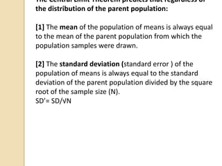
The Central Limit Theorem predicts that regardless of
the distribution of the parent population:
[1] The mean of the population of means is always equal
to the mean of the parent population from which the
population samples were drawn.
[2] The standard deviation (standard error ) of the
population of means is always equal to the standard
deviation of the parent population divided by the square
root of the sample size (N).
SD’= SD/√N
If the population from which samples are drawn is normally distributed then
the sampling distribution of sample means will be normally distributed
regardless of the size of the sample, and the CLT is not needed.
But, if the population is not normal, the CLT tells us that the sampling
distribution of sample means will be normal provided the sample size is
sufficiently large.
How large must the sample size be so that the sampling distribution of
the mean becomes a normal distribution?
If the samples were drawn from a population with a high degree of skewness
(not normal), the sample size must be 30 or more before the sampling
distribution of the mean becomes a normal distribution. A sample of size 30
or more is called a large sample and as a sample of size less that thirty is
called a small sample.