Downloaded 793 times


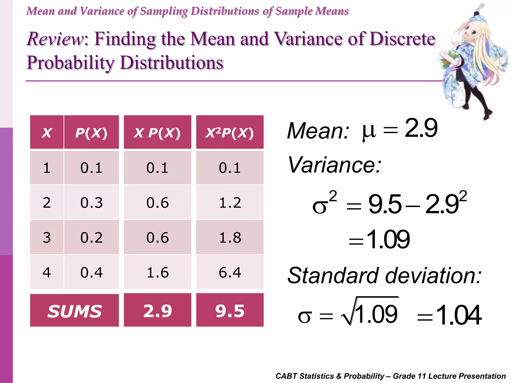
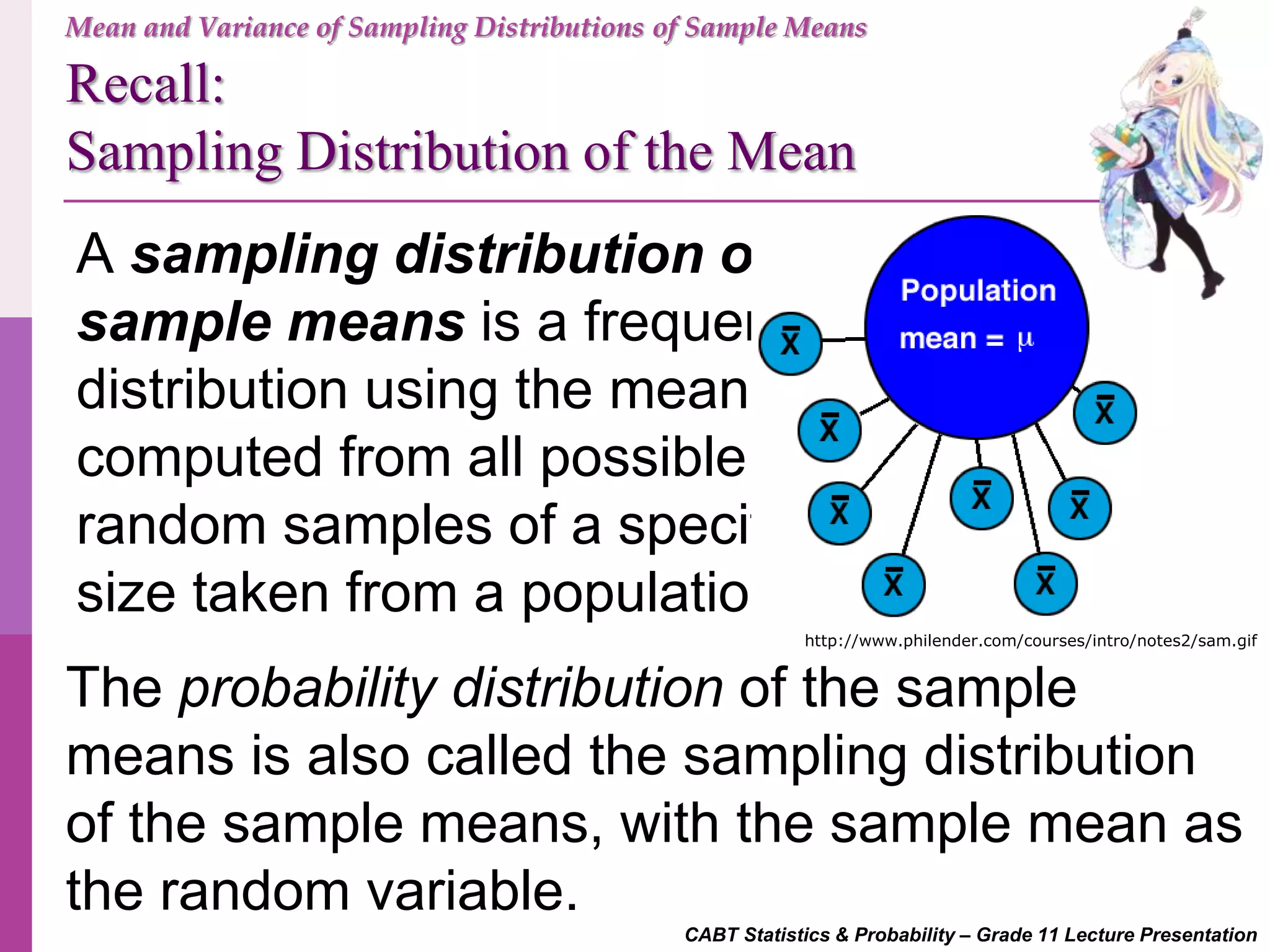

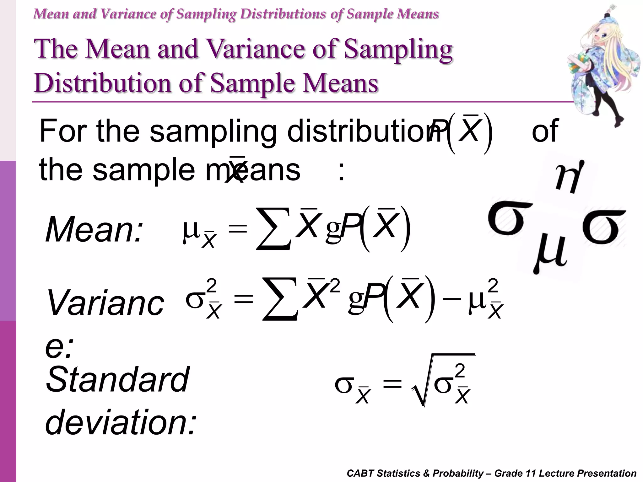
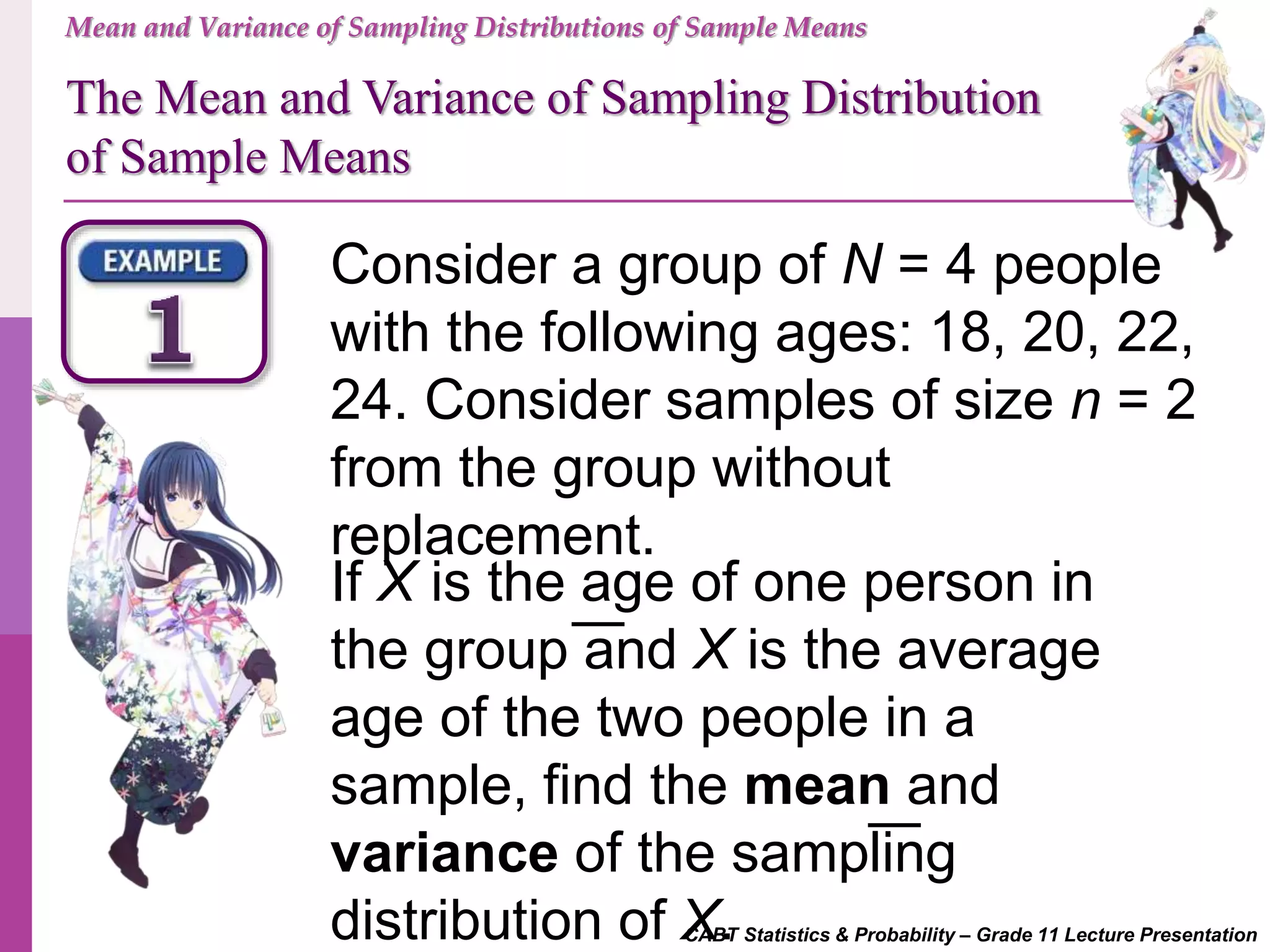
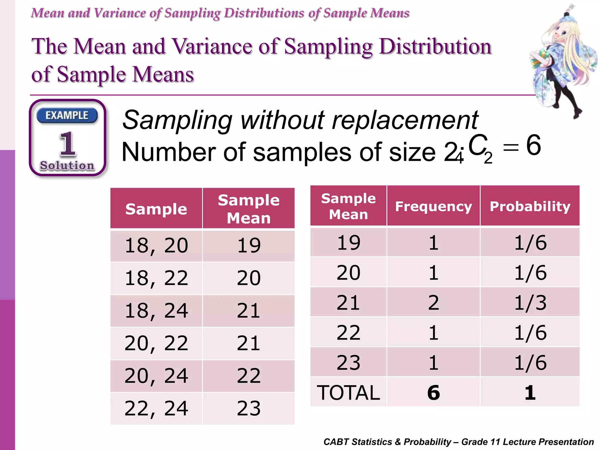
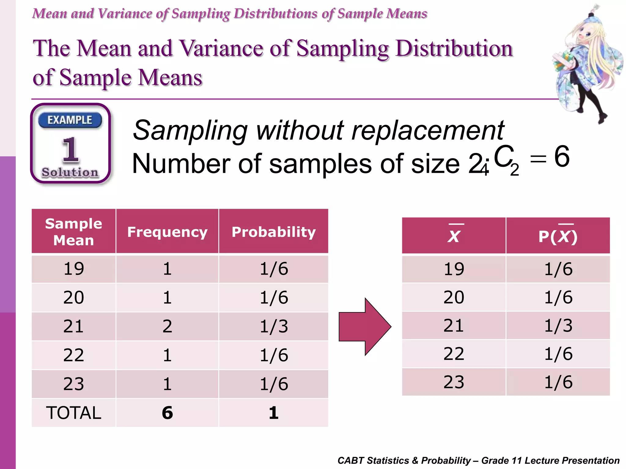
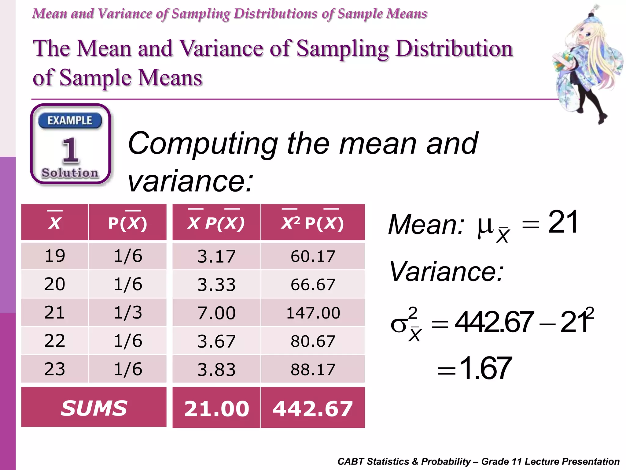
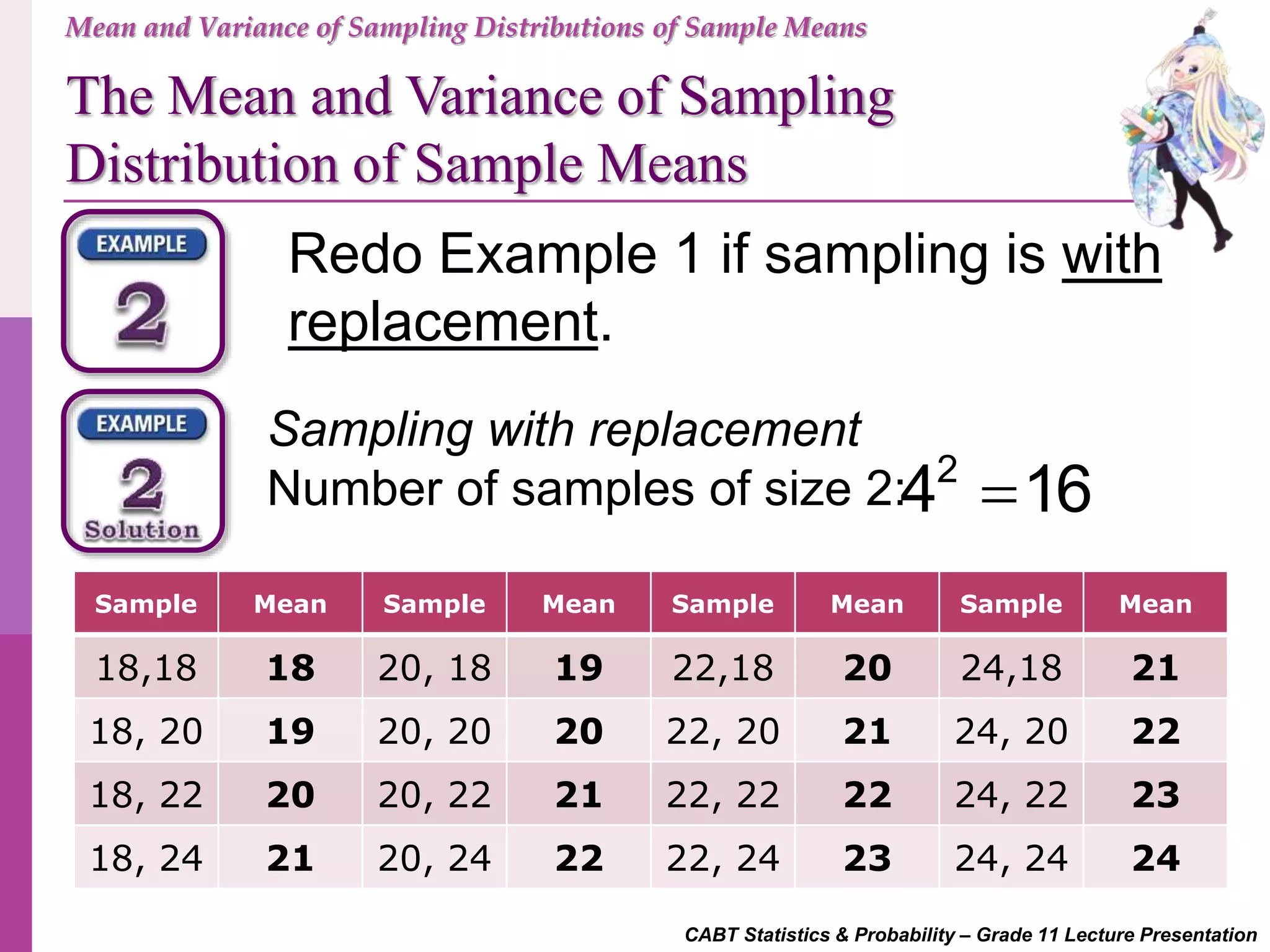
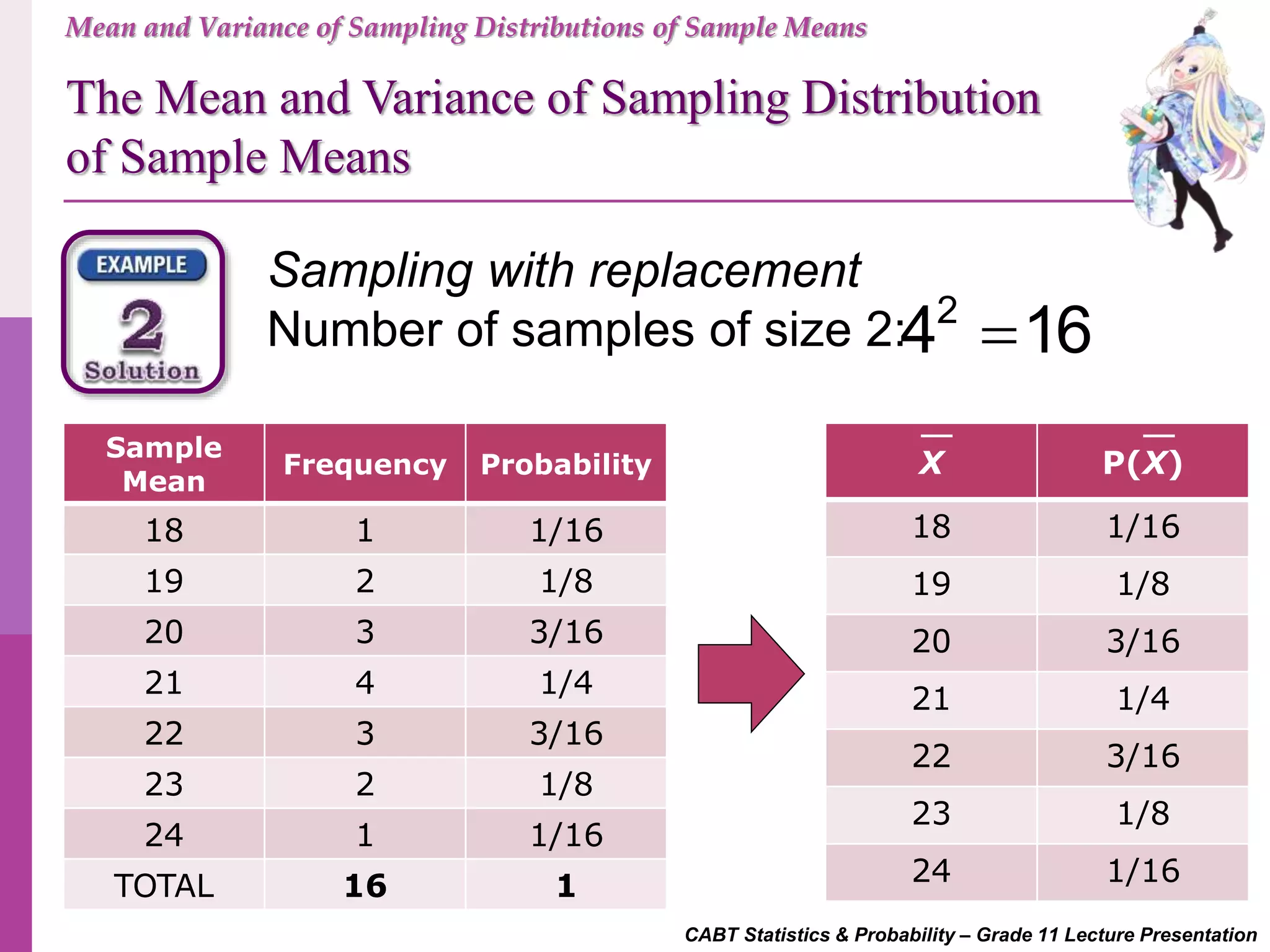


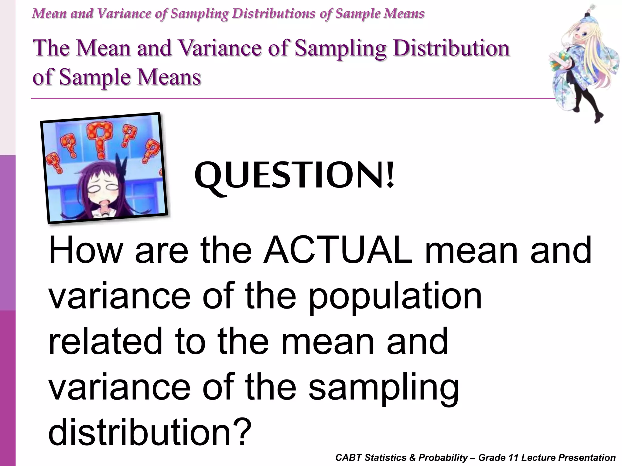
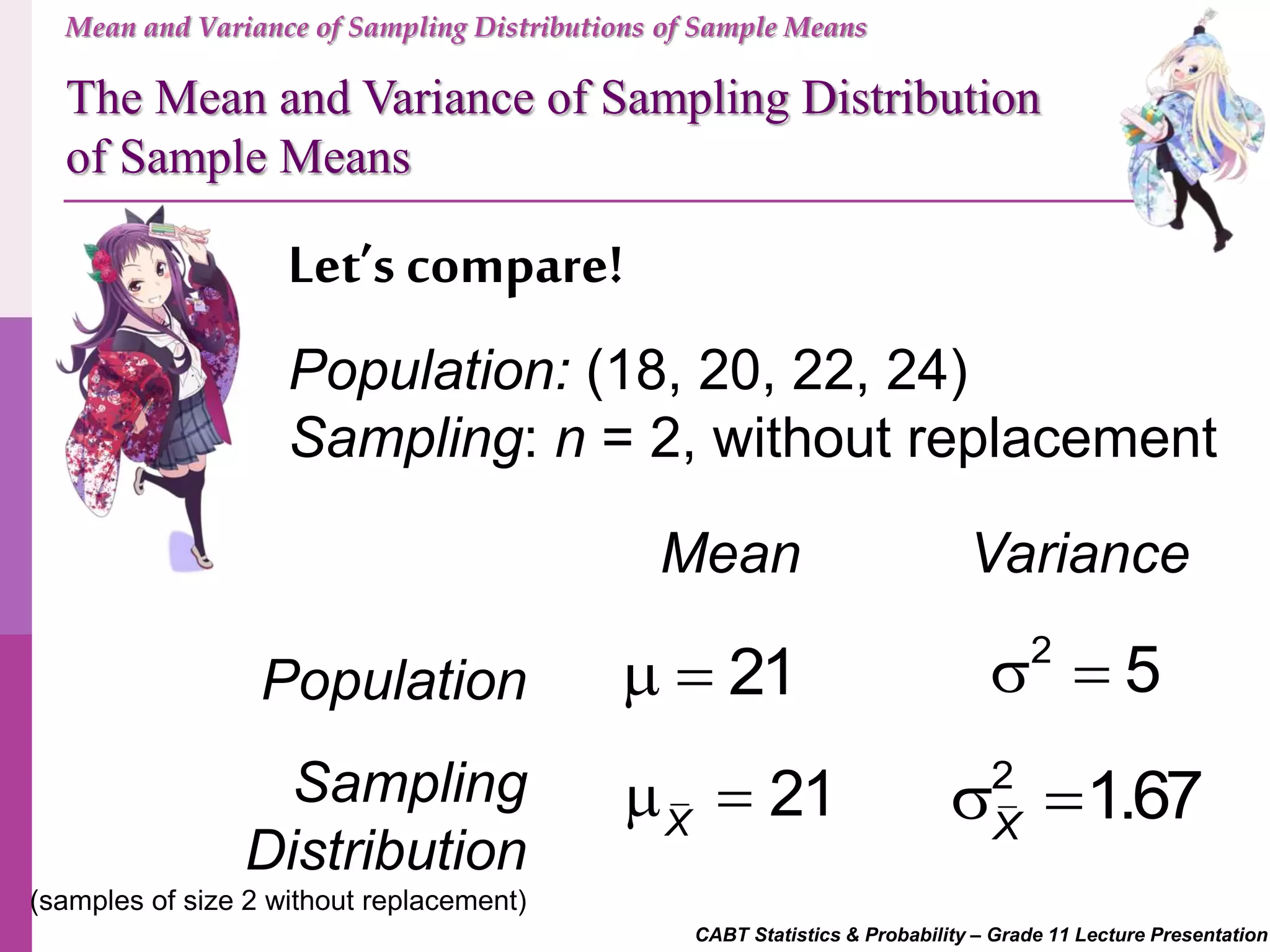
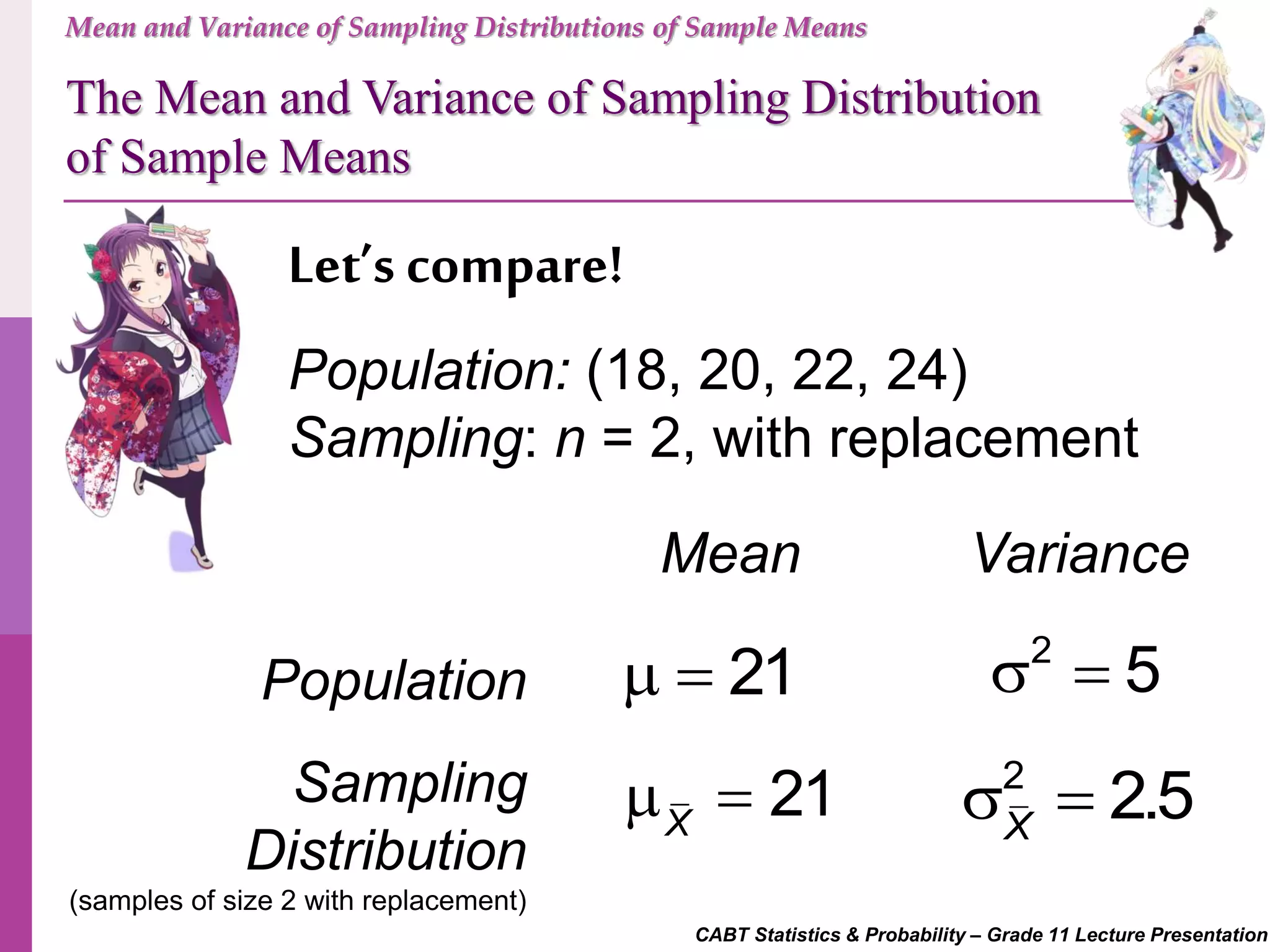
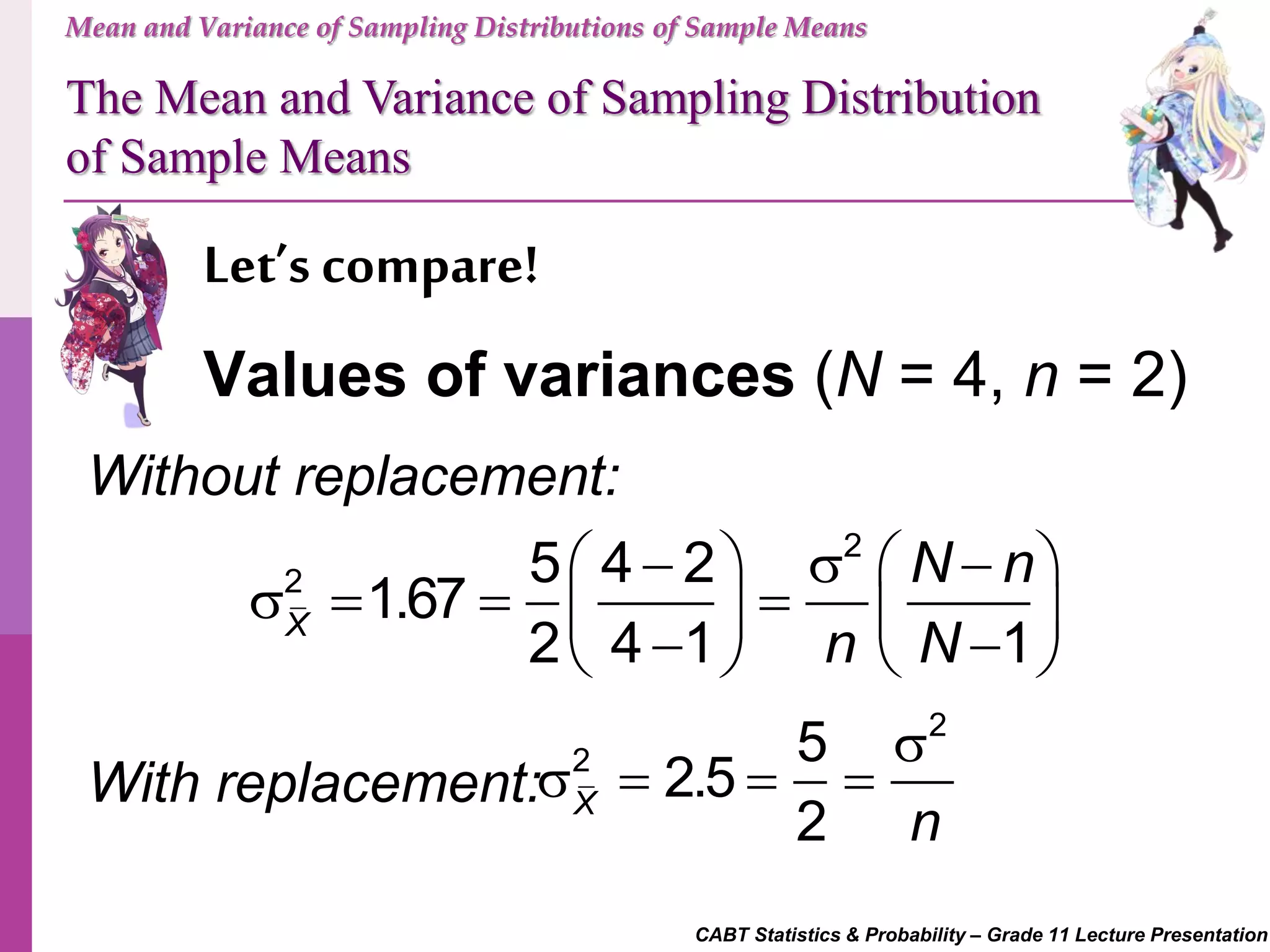
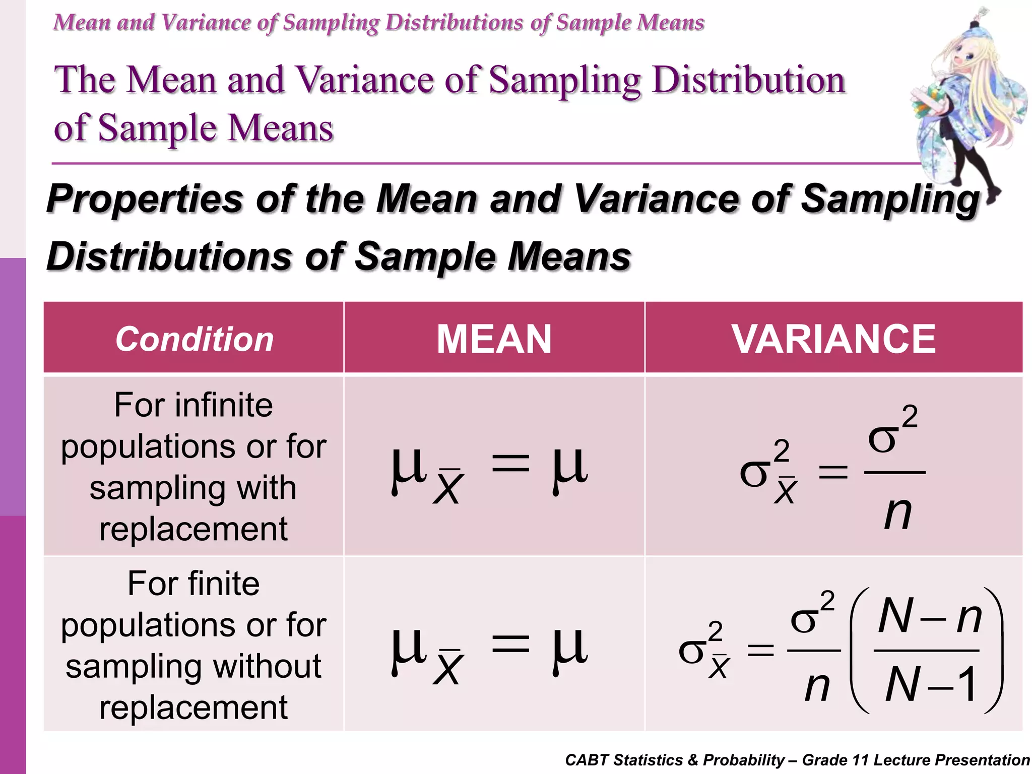
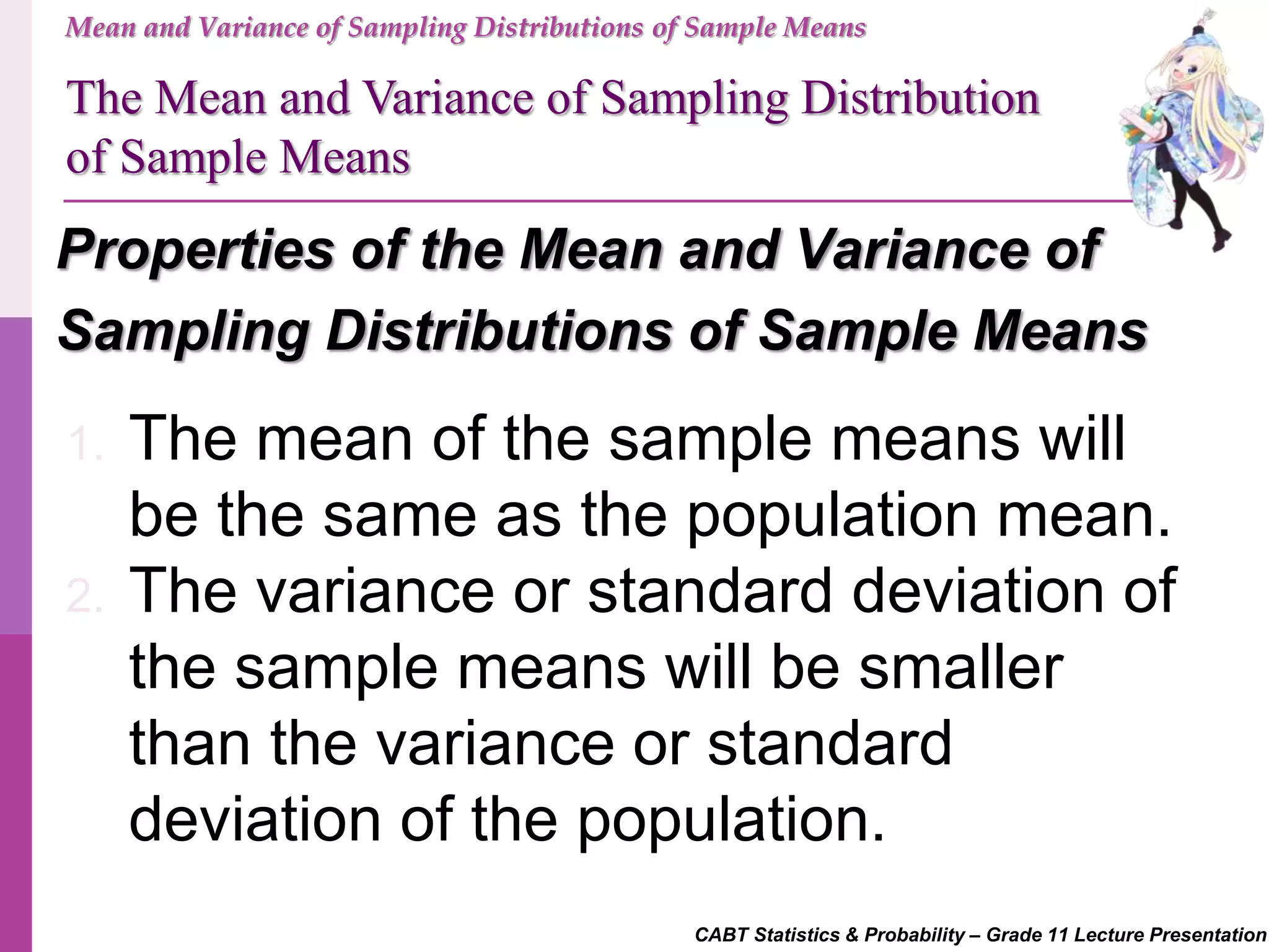
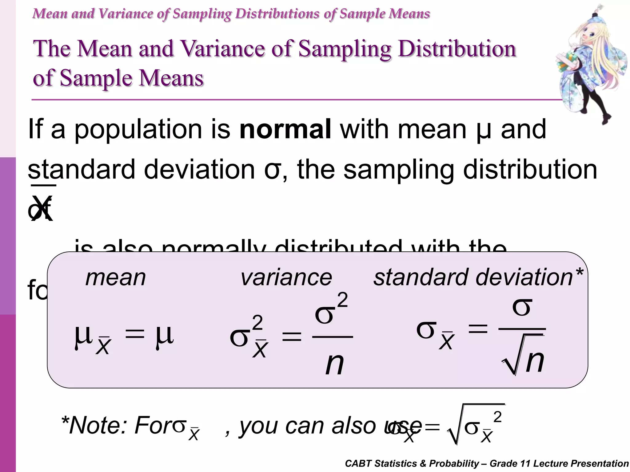
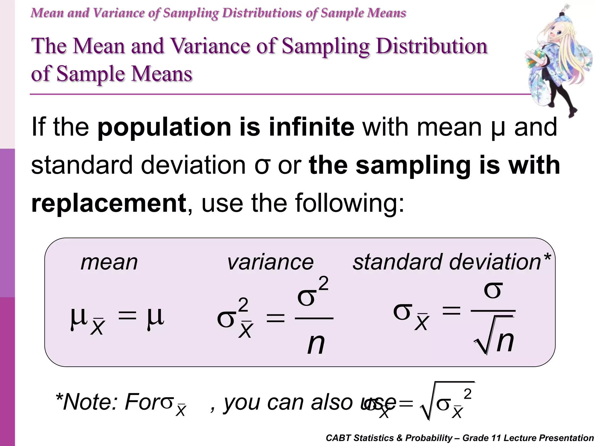
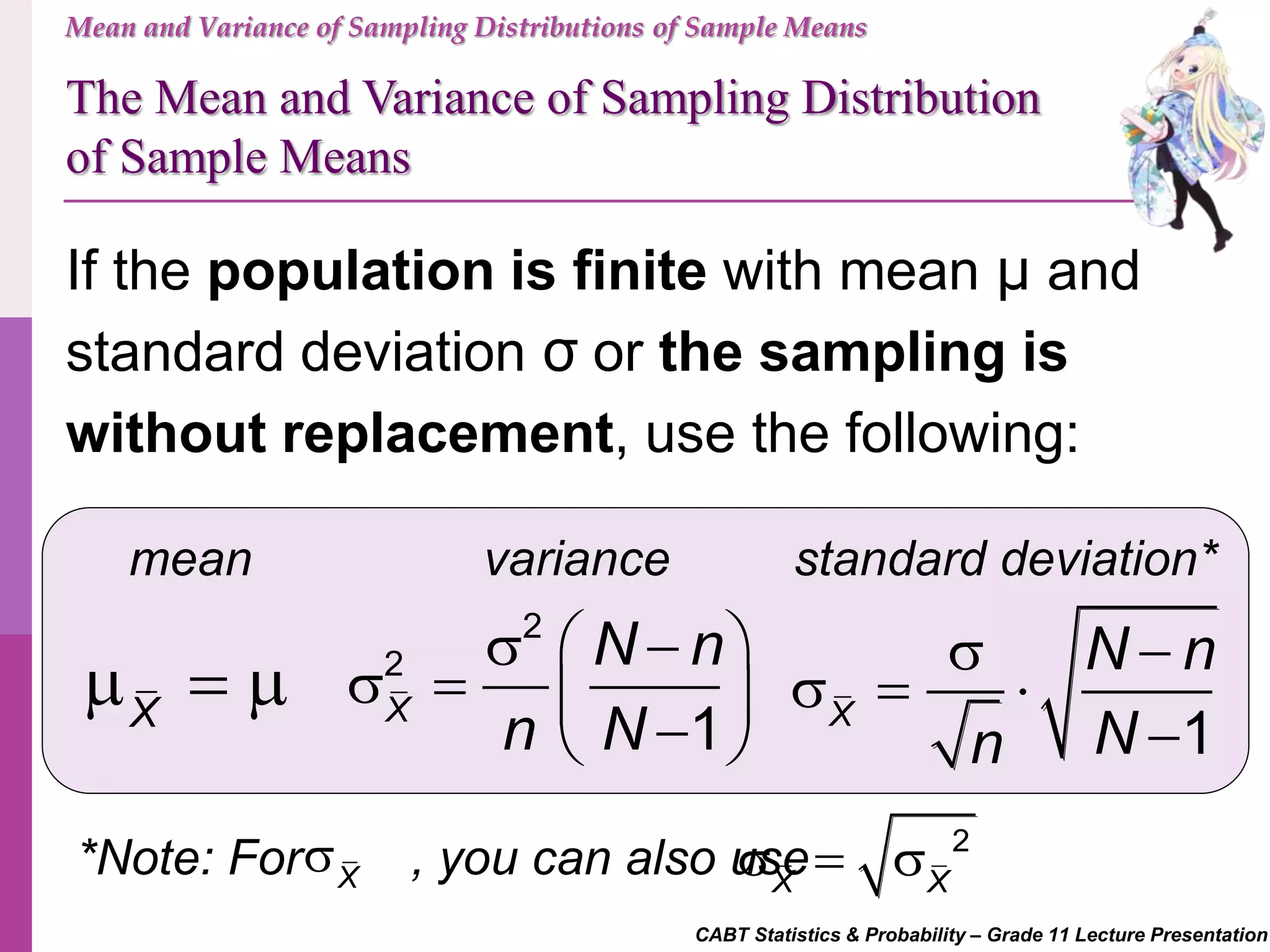
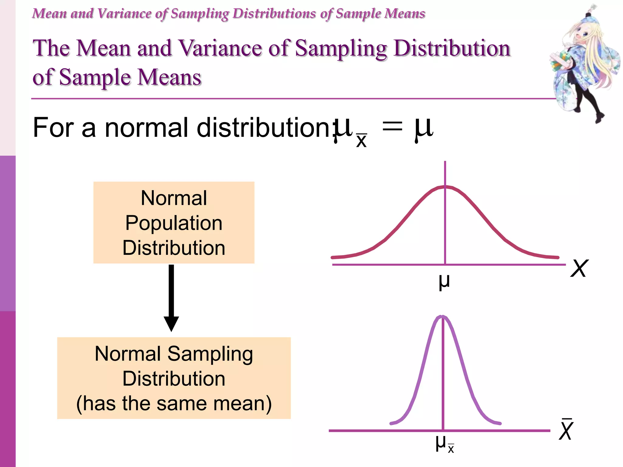
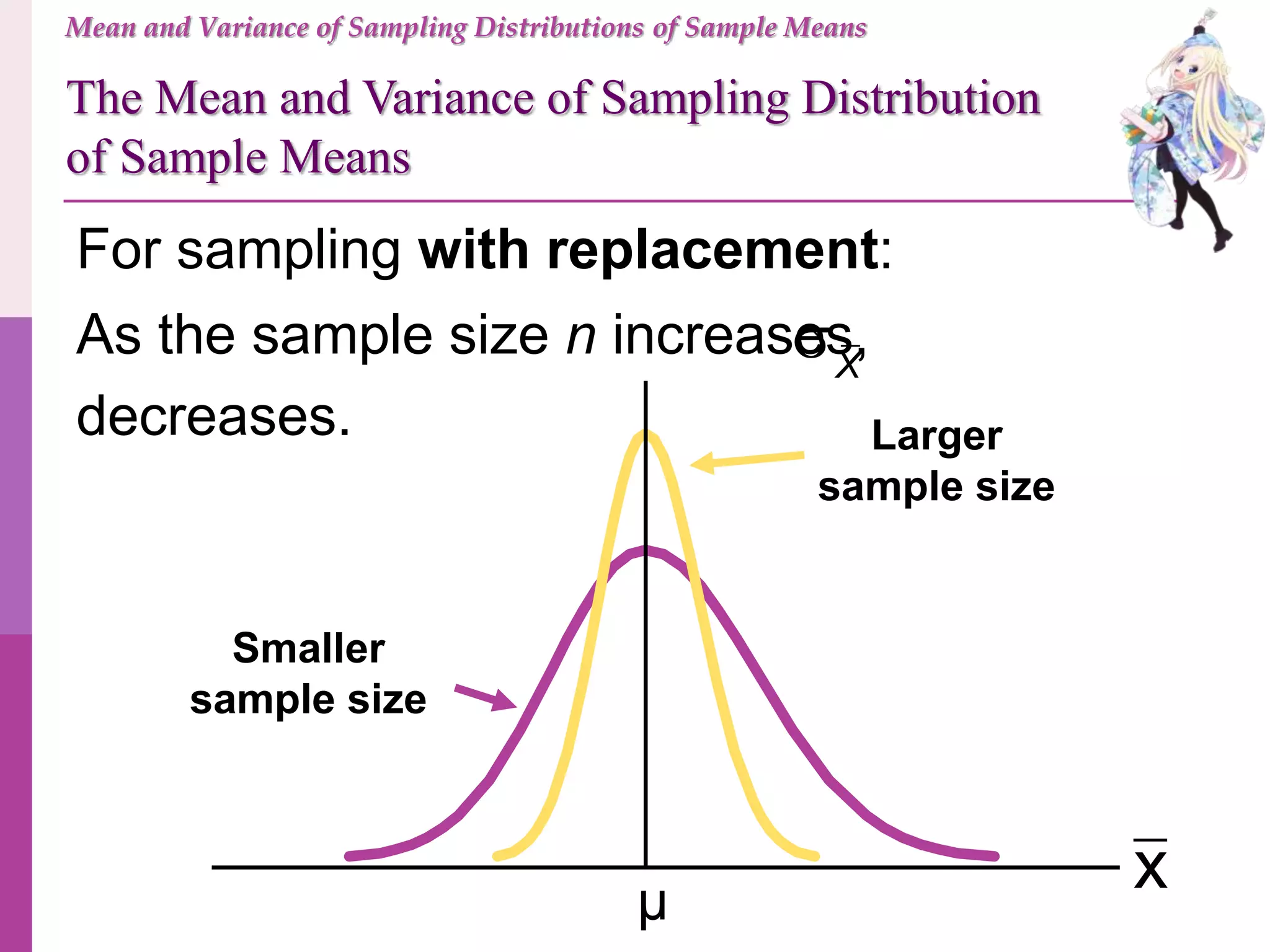
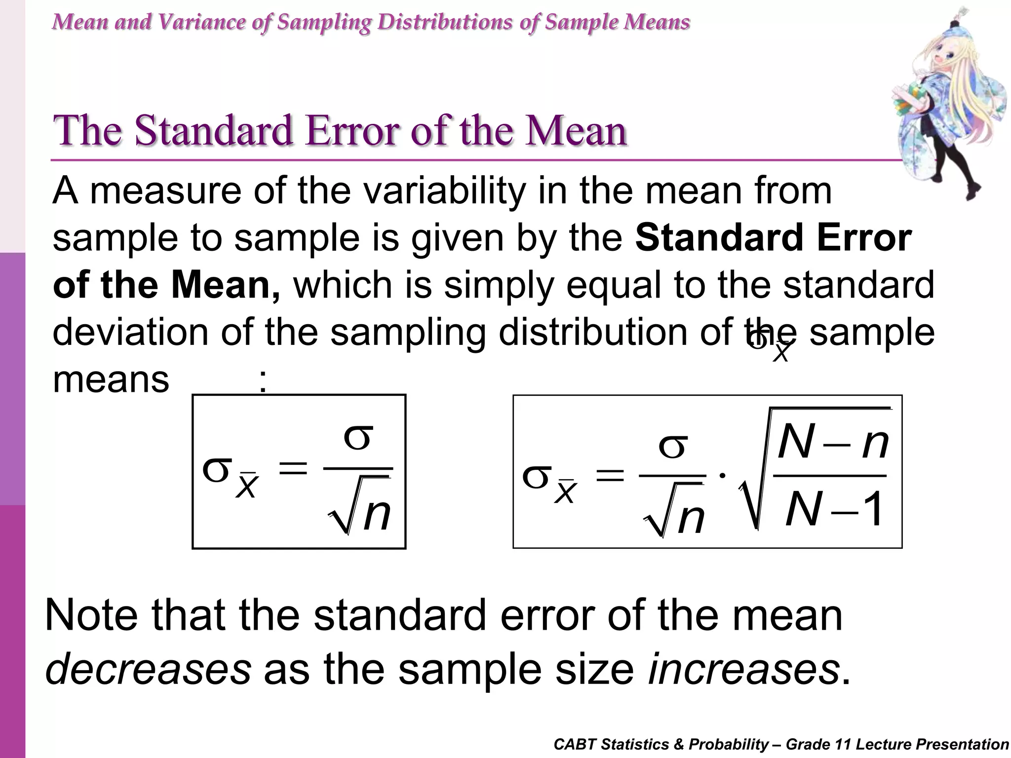
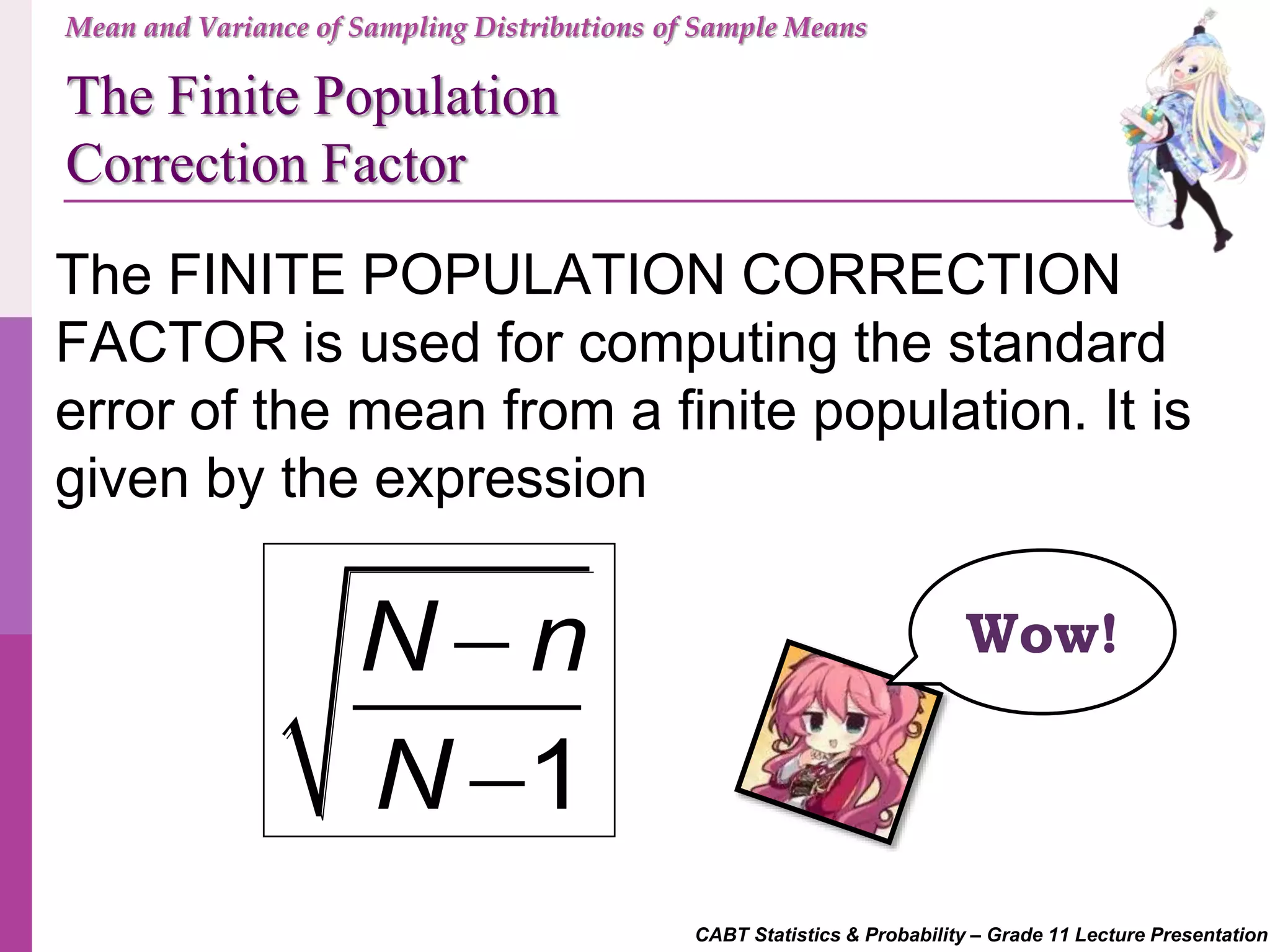
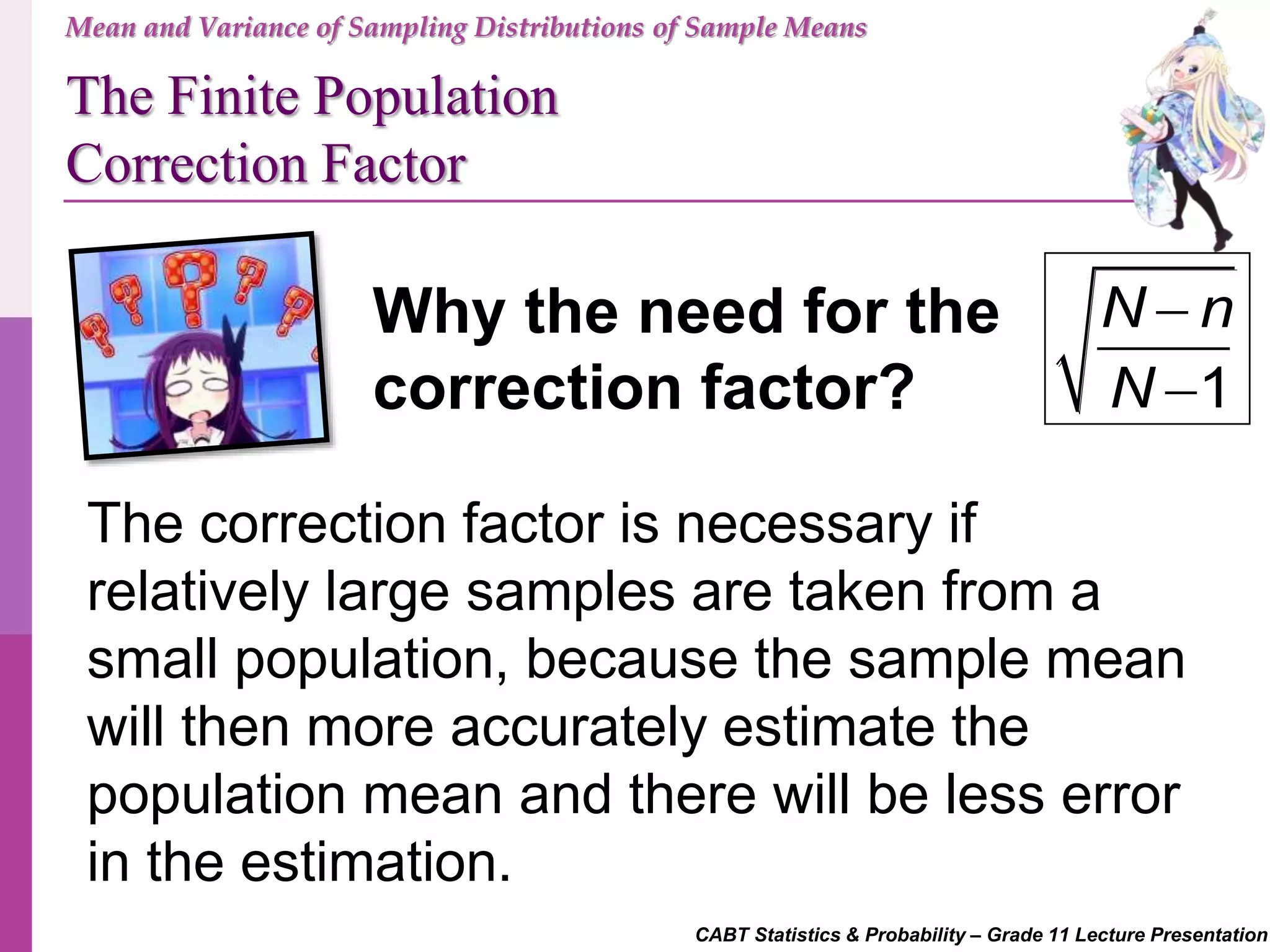
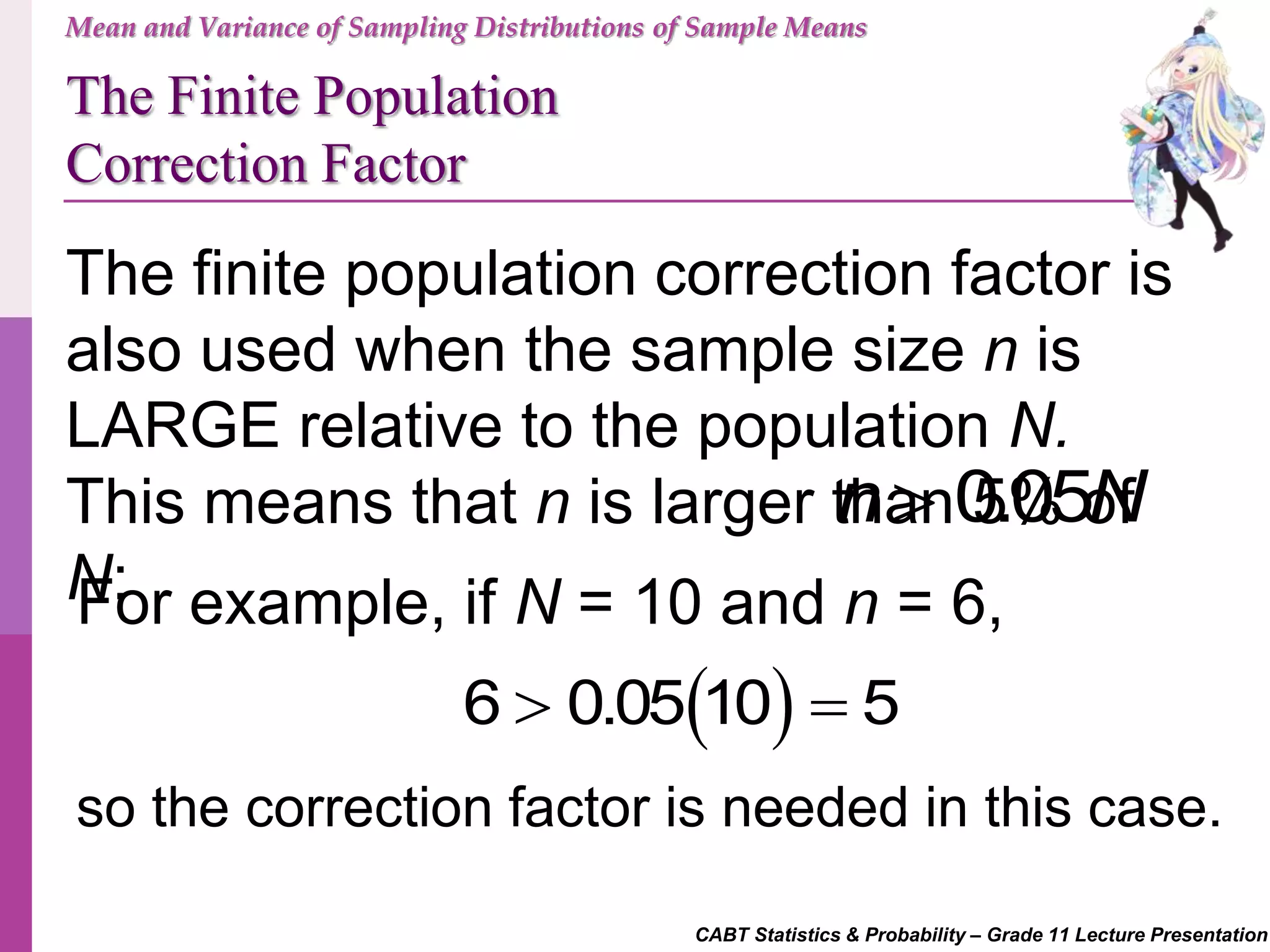
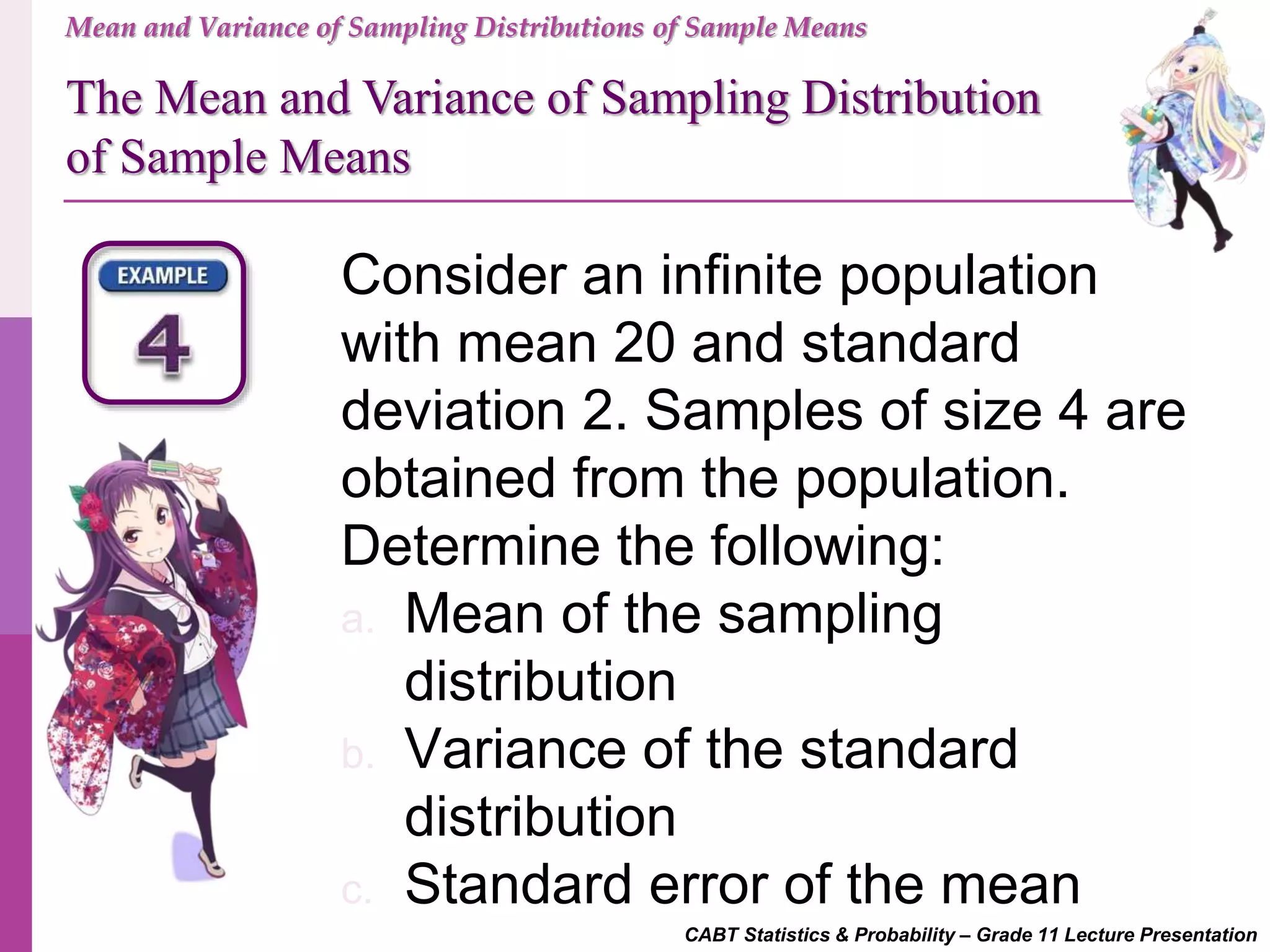
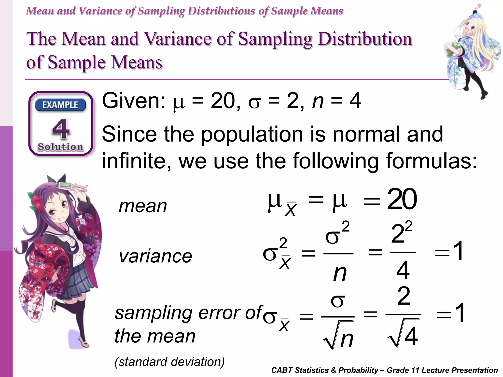


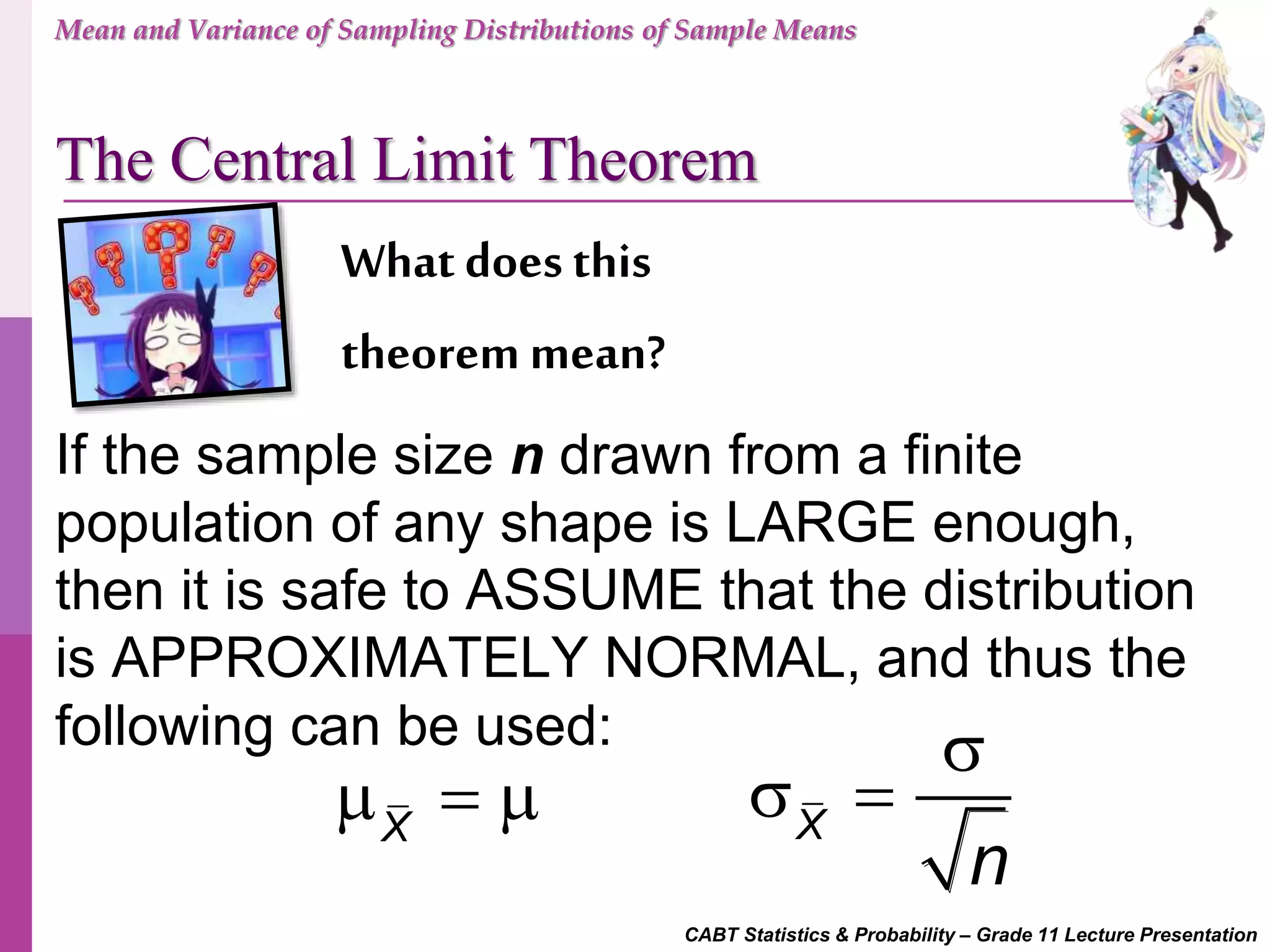
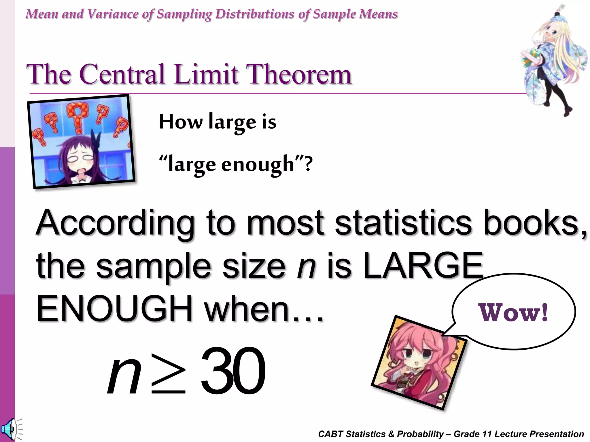
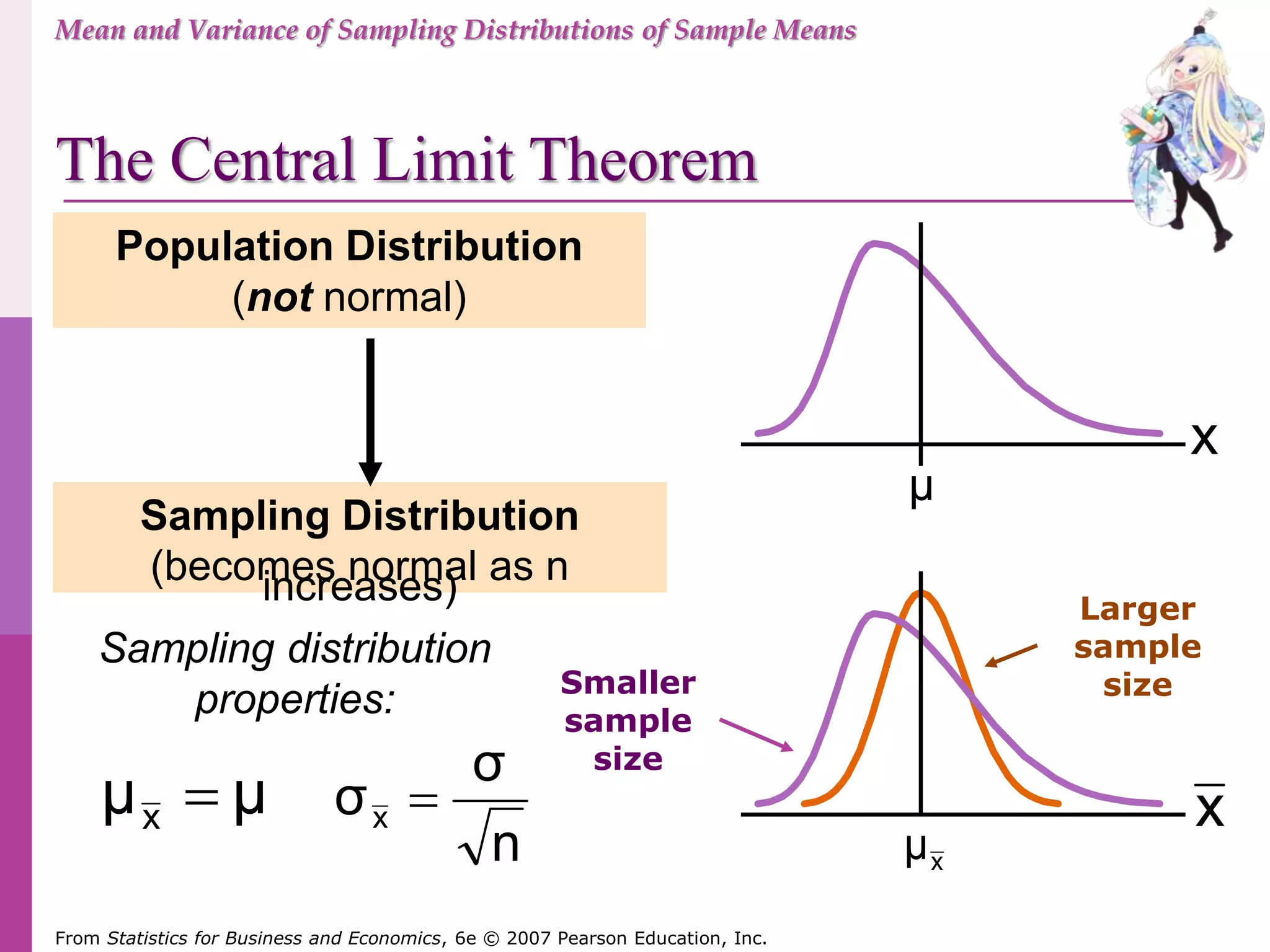
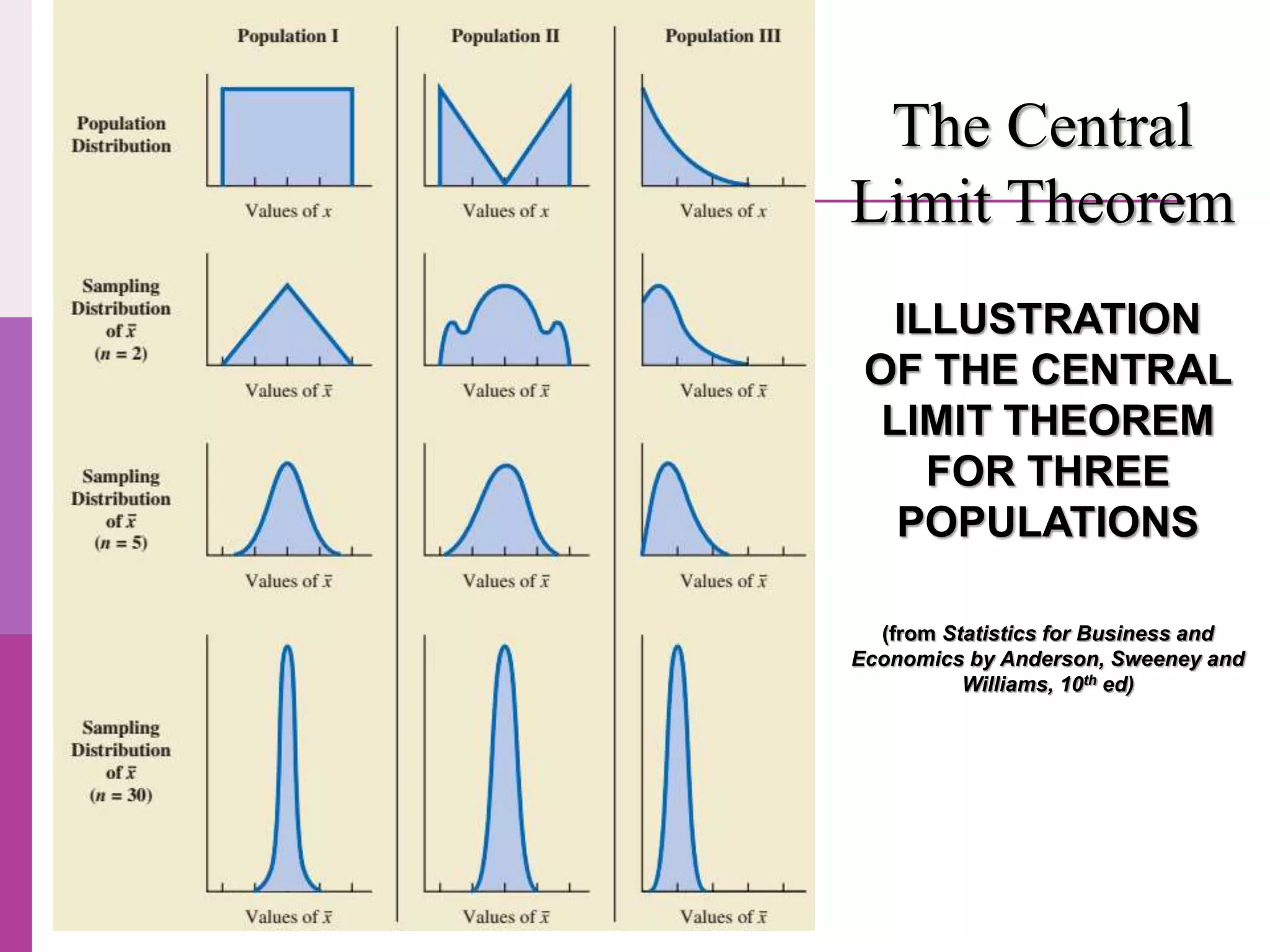


The document is a Grade 11 statistics lecture presentation that covers the mean and variance of sampling distributions of sample means. It explains the central limit theorem and provides examples of constructing sampling distributions and calculating their mean and variance for finite and infinite populations. Additionally, it discusses the effects of sampling with and without replacement, and introduces the finite population correction factor.