Downloaded 348 times


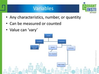
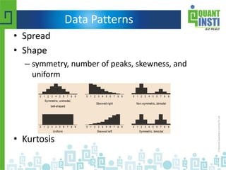
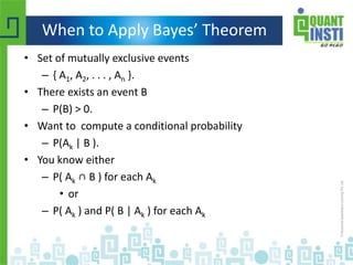
![Standard Deviation
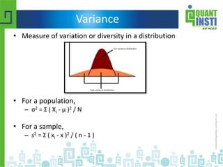
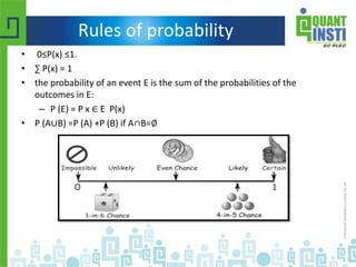
• For a population
– σ = sqrt[ σ2 ] = sqrt [ Σ ( Xi - μ )2 / N ]
• For a sample
– s = sqrt[ s2 ] = sqrt [ Σ ( xi - x )2 / ( n - 1 ) ]](https://image.slidesharecdn.com/basicstatisticsforalgorithmictrading-150513122821-lva1-app6892/85/Basic-statistics-for-algorithmic-trading-13-320.jpg)
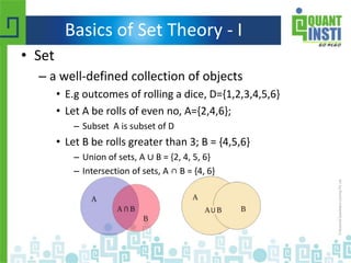


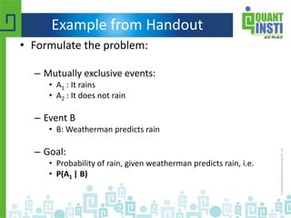
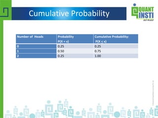


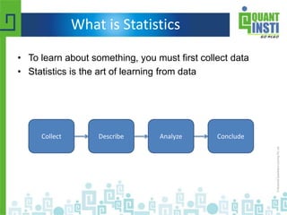
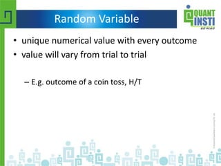
![Binomial Distribution
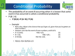
Number of heads Probability
0 0.25
1 0.50
2 0.25
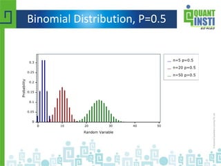
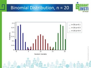
The mean of the distribution (μx) is equal to n * P .
The variance (σ2
x) is n * P * ( 1 - P )
The standard deviation (σx) is sqrt[ n * P * ( 1 - P ) ].](https://image.slidesharecdn.com/basicstatisticsforalgorithmictrading-150513122821-lva1-app6892/85/Basic-statistics-for-algorithmic-trading-34-320.jpg)


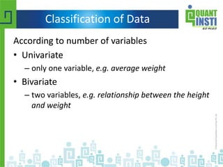
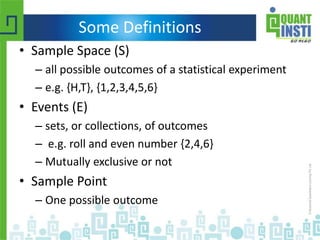
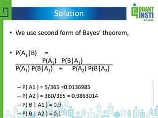
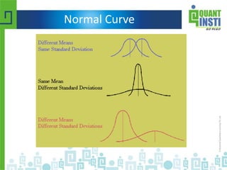
![Normal Distribution
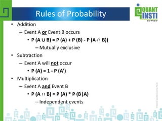
X = { 1/[ σ * sqrt(2π) ] } * e^(-(x-μ)^2 /2 /σ^2 )](https://image.slidesharecdn.com/basicstatisticsforalgorithmictrading-150513122821-lva1-app6892/85/Basic-statistics-for-algorithmic-trading-41-320.jpg)


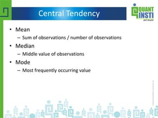
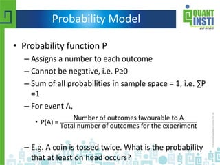
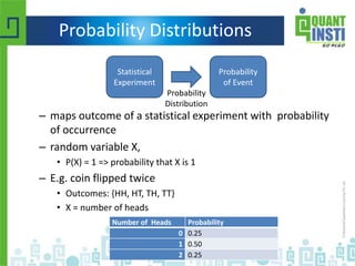
![Student's t Distribution
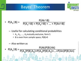
• t = [x - μ] / [s / sqrt( n ) ]
• Small sample sizes](https://image.slidesharecdn.com/basicstatisticsforalgorithmictrading-150513122821-lva1-app6892/85/Basic-statistics-for-algorithmic-trading-48-320.jpg)

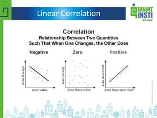
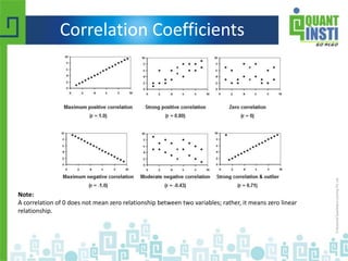
![Correlation Coefficients
• Measure the strength of association between two
variables
• Pearson product-moment correlation coefficient
r = Σ (xy) / sqrt[ ( Σ x2 ) * ( Σ y2 ) ]
– x = xi - x,
– xi is the x value for observation i
– x is the mean x value,
– y = yi – y
– yi is the y value for observation I
– y is the mean y value.](https://image.slidesharecdn.com/basicstatisticsforalgorithmictrading-150513122821-lva1-app6892/85/Basic-statistics-for-algorithmic-trading-58-320.jpg)
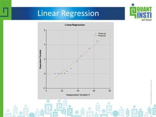
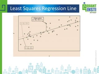
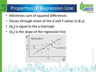
![Regression line
• ŷ = b0 + b1x
– b1 = Σ [ (xi - x)(yi - y) ] / Σ [ (xi - x)2]
– b1 = r * (sy / sx)
– b0 = y - b1 * x
• b0 is the constant in the regression equation
• b1 is the regression coefficient
• r is the correlation between x and y
• xi is the X value of observation I
• yi is the Y value of observation I
• x is the mean of X
• y is the mean of Y
• sx is the standard deviation of X
• sy is the standard deviation of Y](https://image.slidesharecdn.com/basicstatisticsforalgorithmictrading-150513122821-lva1-app6892/85/Basic-statistics-for-algorithmic-trading-62-320.jpg)
![Coefficient of Determination
• R2
– Between 0 and 1
– R2 = 0, dependent variable cannot be predicted
– R2 = 1, dependent variable can be predicted without error
– An R2 between 0 and 1 indicates the extent to which the
dependent variable is predictable.
• R2 = 0.10 means that 10% of the variance in Y is predictable from X
• R2 = 0.20 means that 20% is predictable
R2 = { ( 1 / N ) * Σ [ (xi - x) * (yi - y) ] / (σx * σy ) }2](https://image.slidesharecdn.com/basicstatisticsforalgorithmictrading-150513122821-lva1-app6892/85/Basic-statistics-for-algorithmic-trading-64-320.jpg)


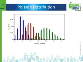
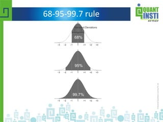
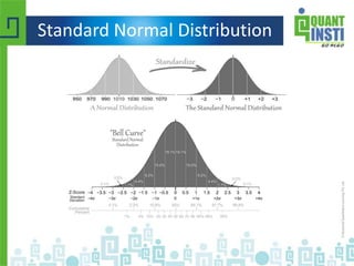
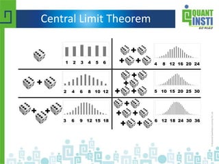
The document provides an extensive overview of basic statistics, including data collection, descriptive and inferential statistics, probability concepts, and types of probability distributions like binomial and Poisson distributions. It explains central tendency measures, variability, correlation, regression analysis, hypothesis testing, and the principles of set theory. Additionally, the document touches on the importance of the normal distribution and its applications in statistical inference and confidence intervals.