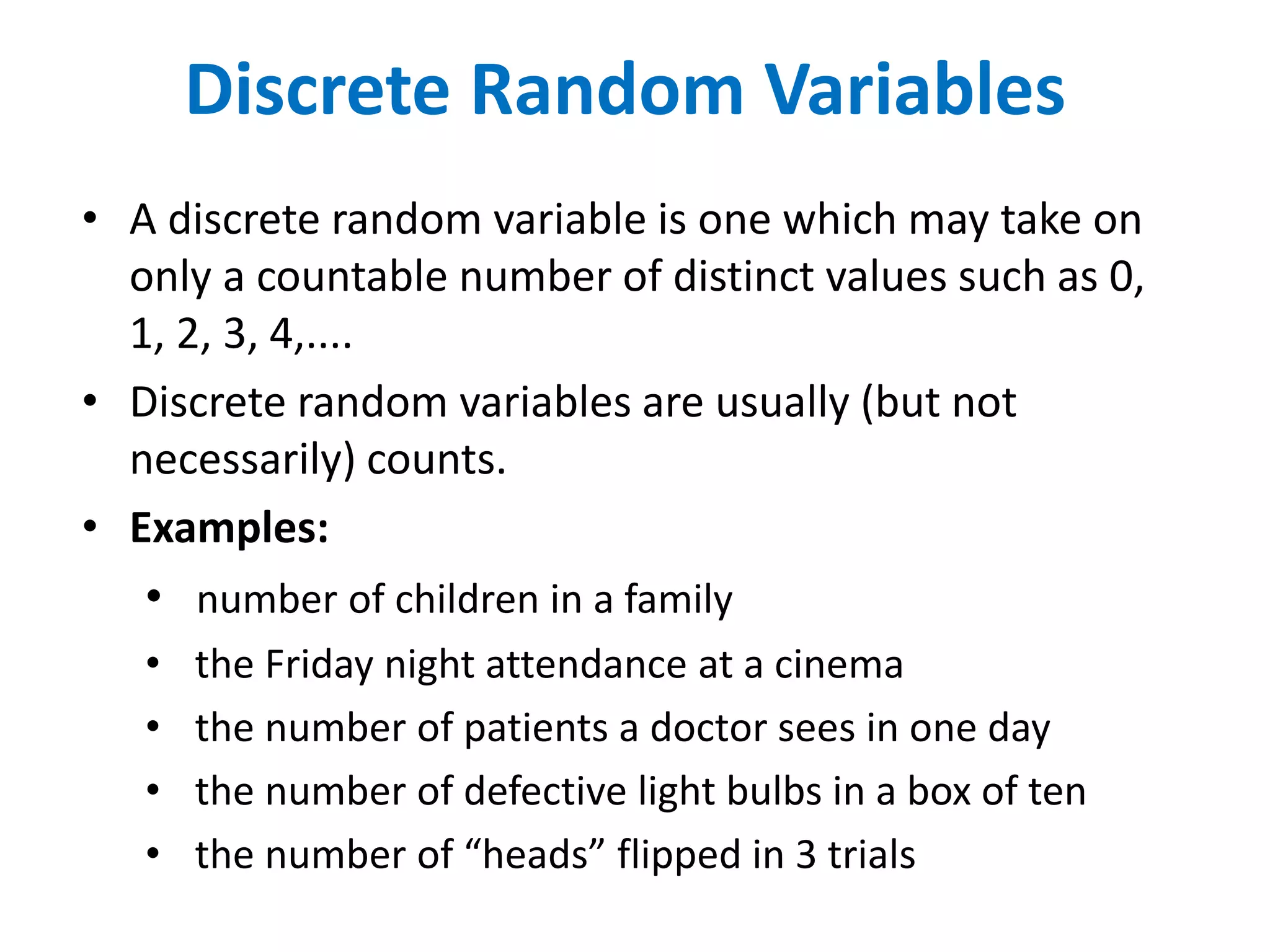
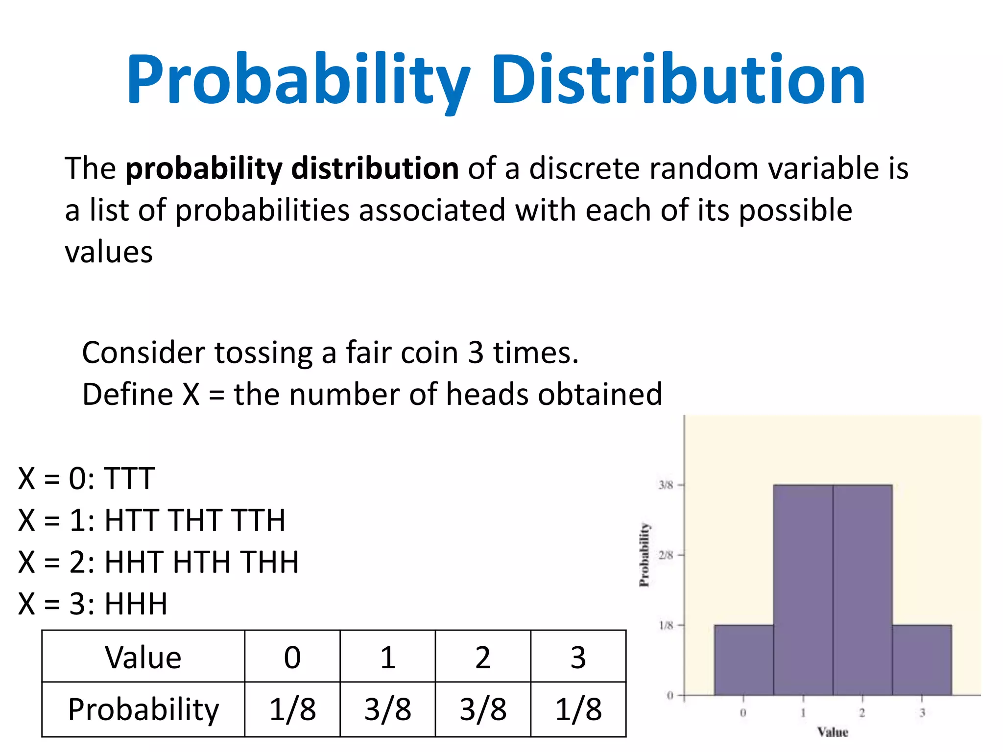
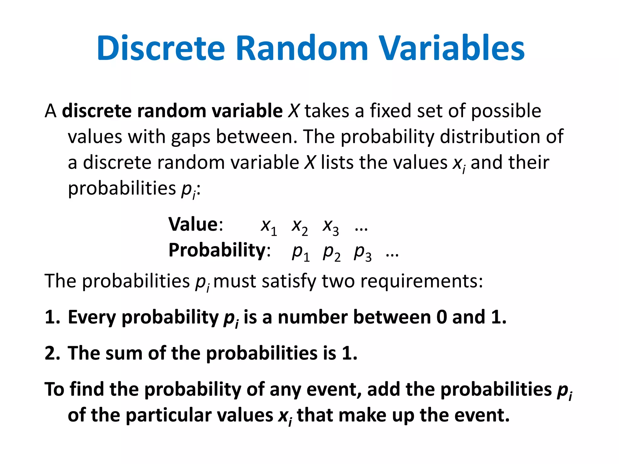
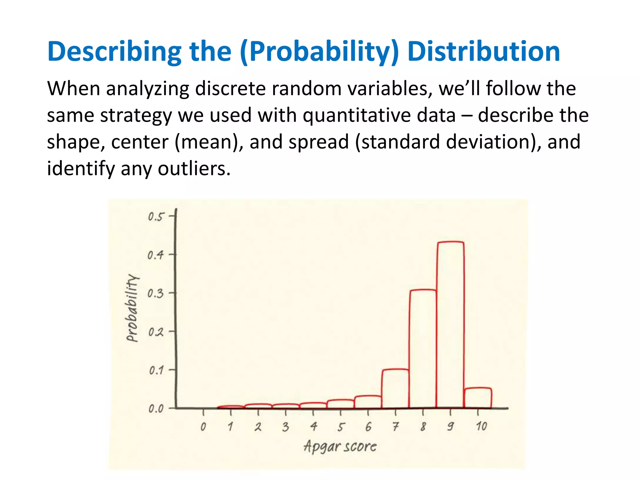
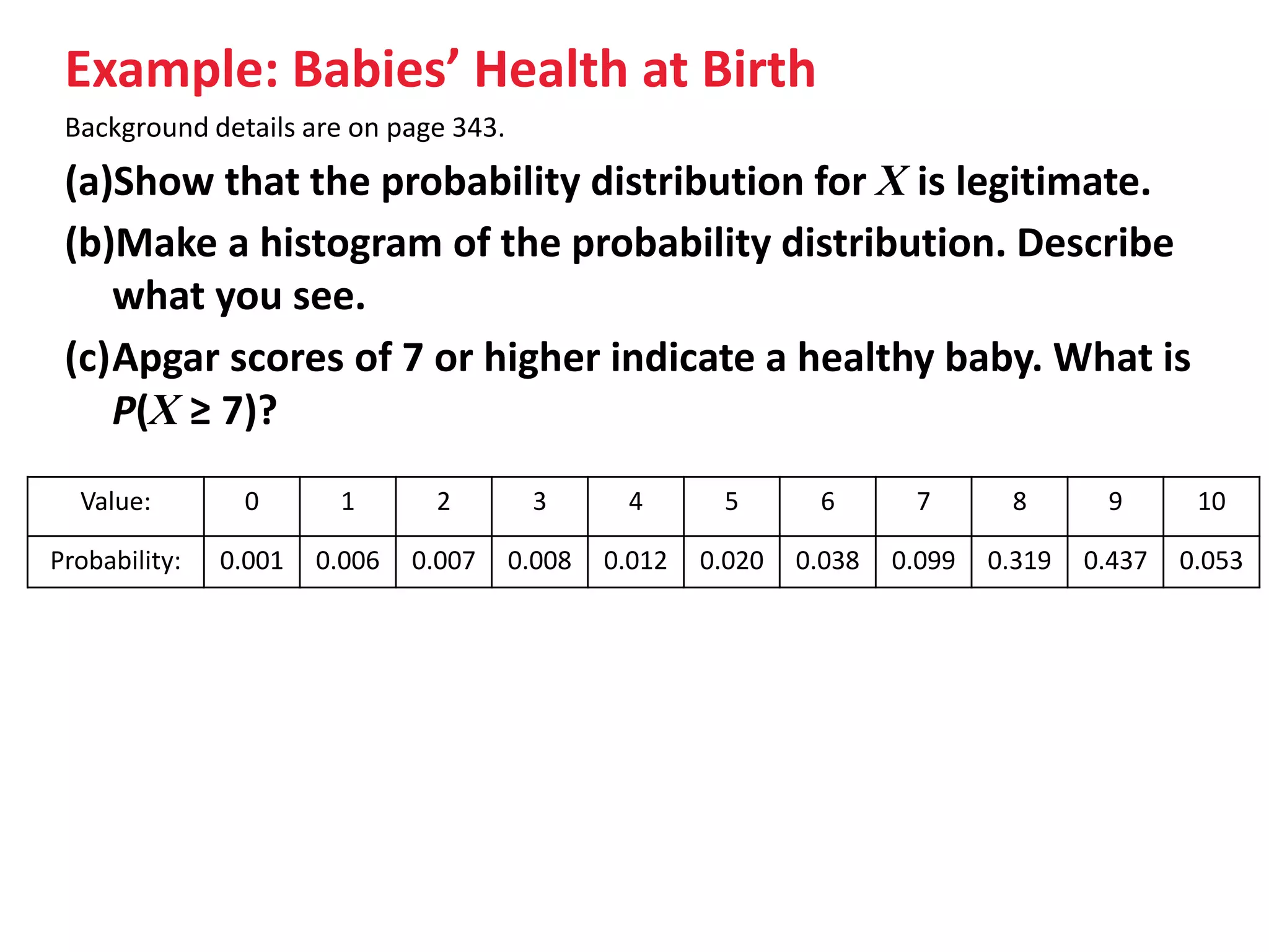
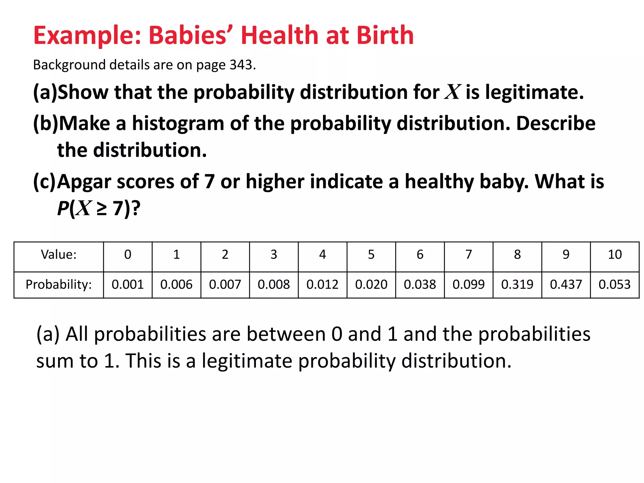
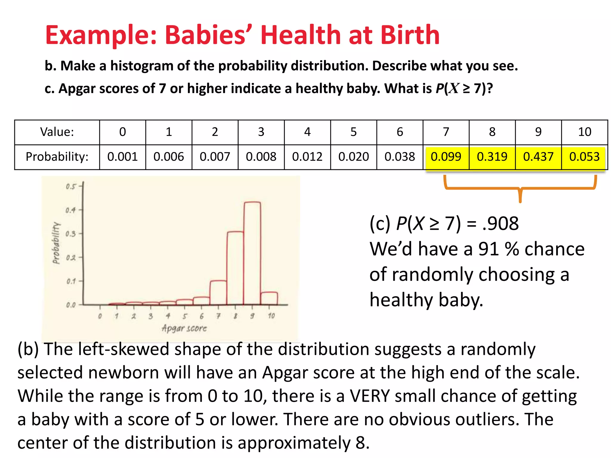
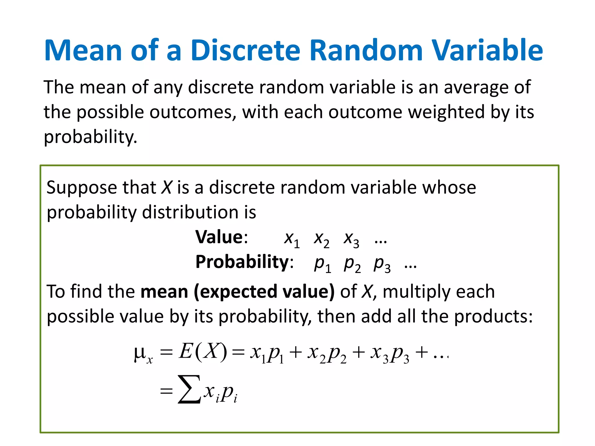
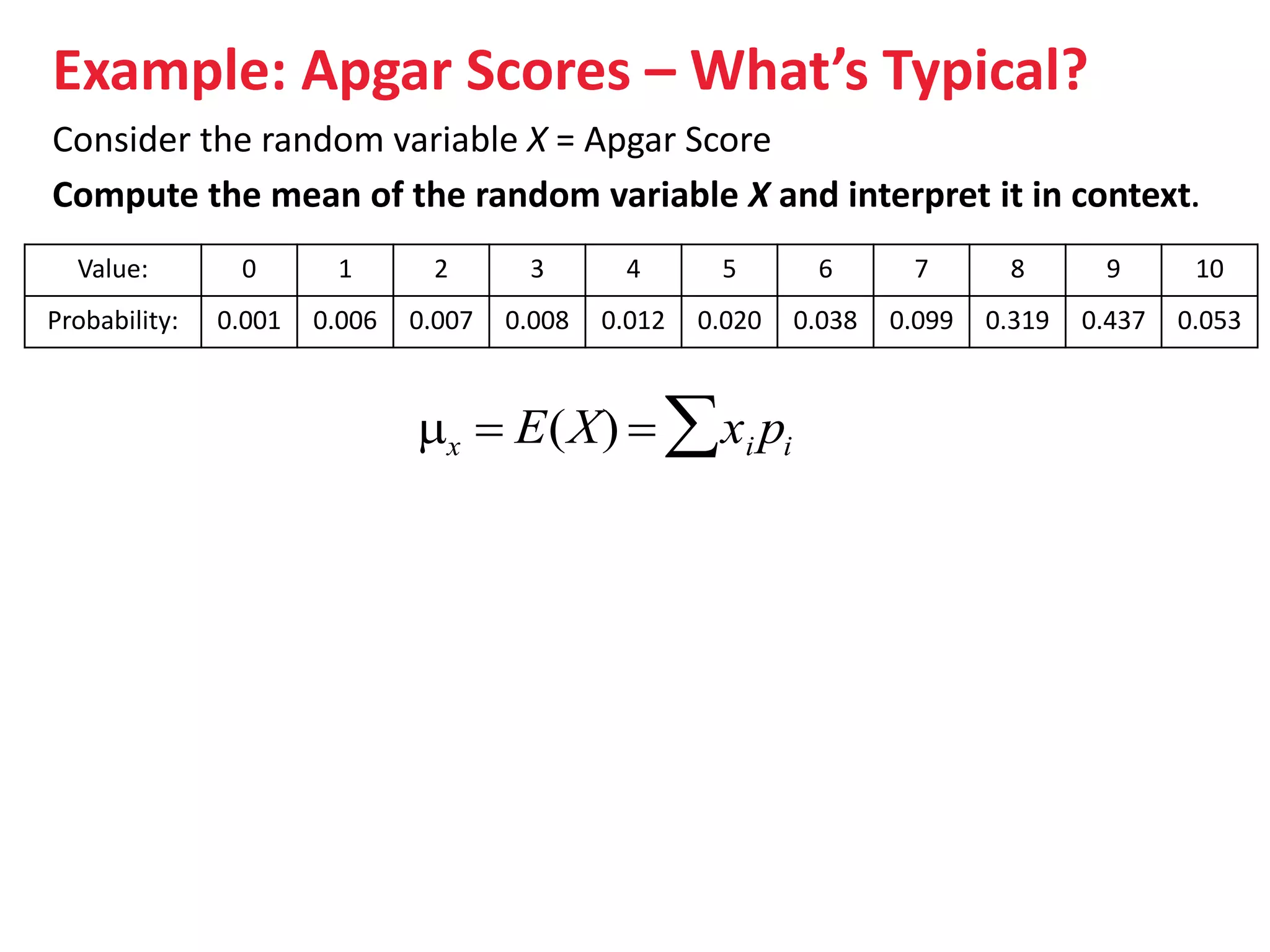
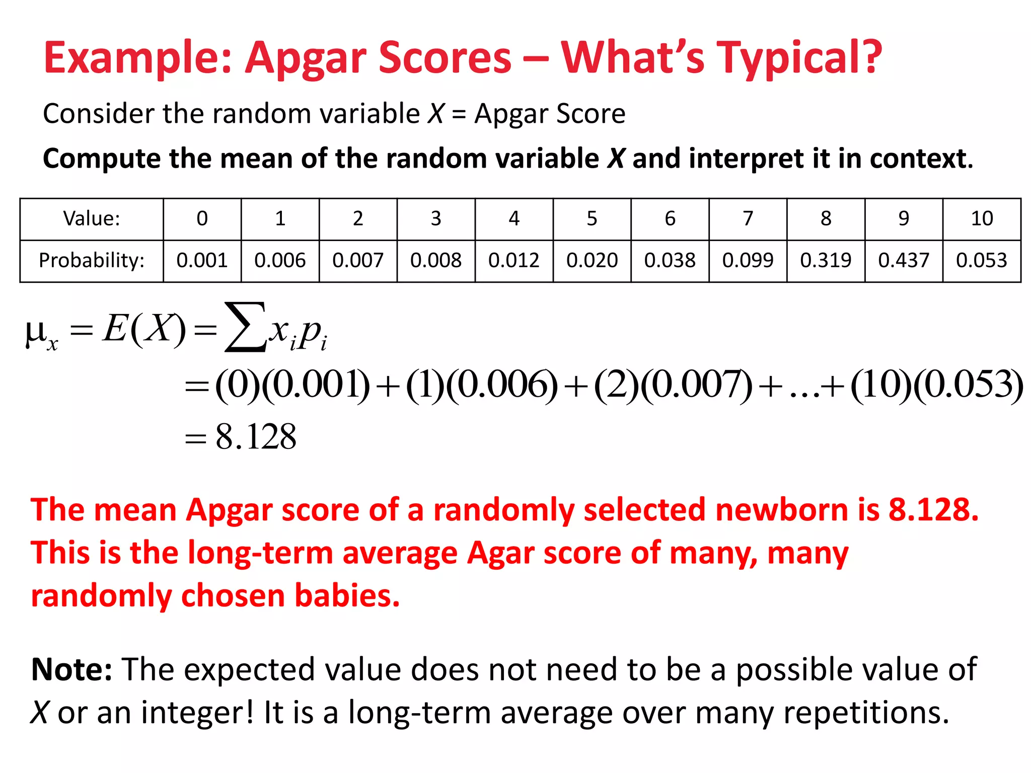
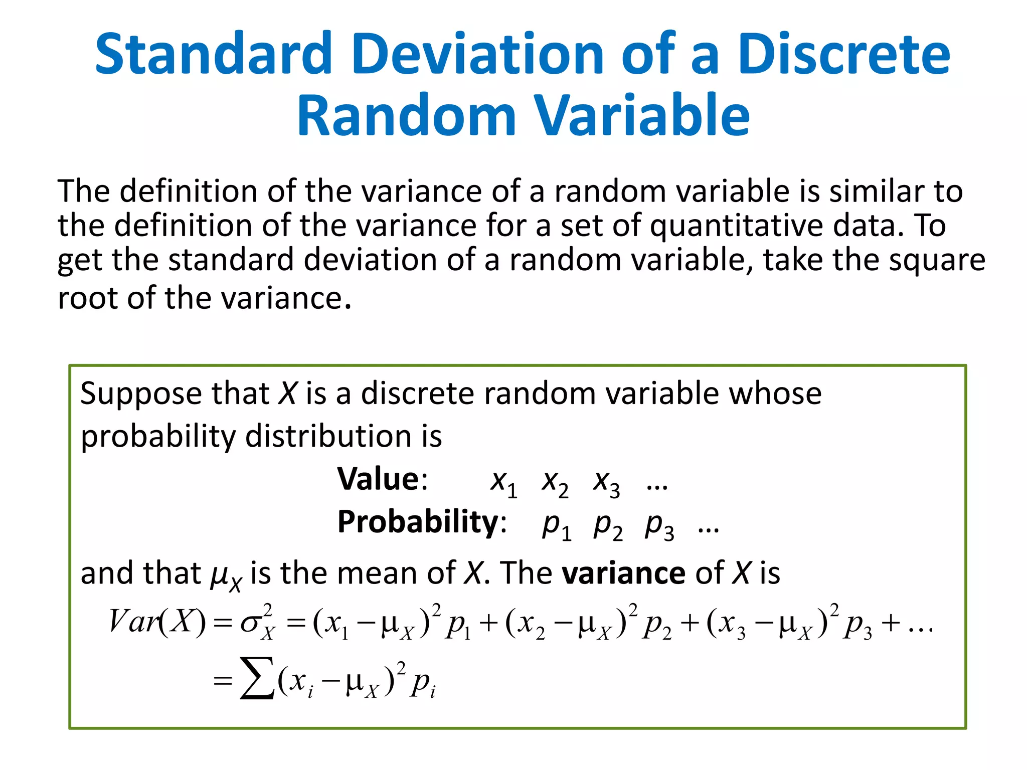
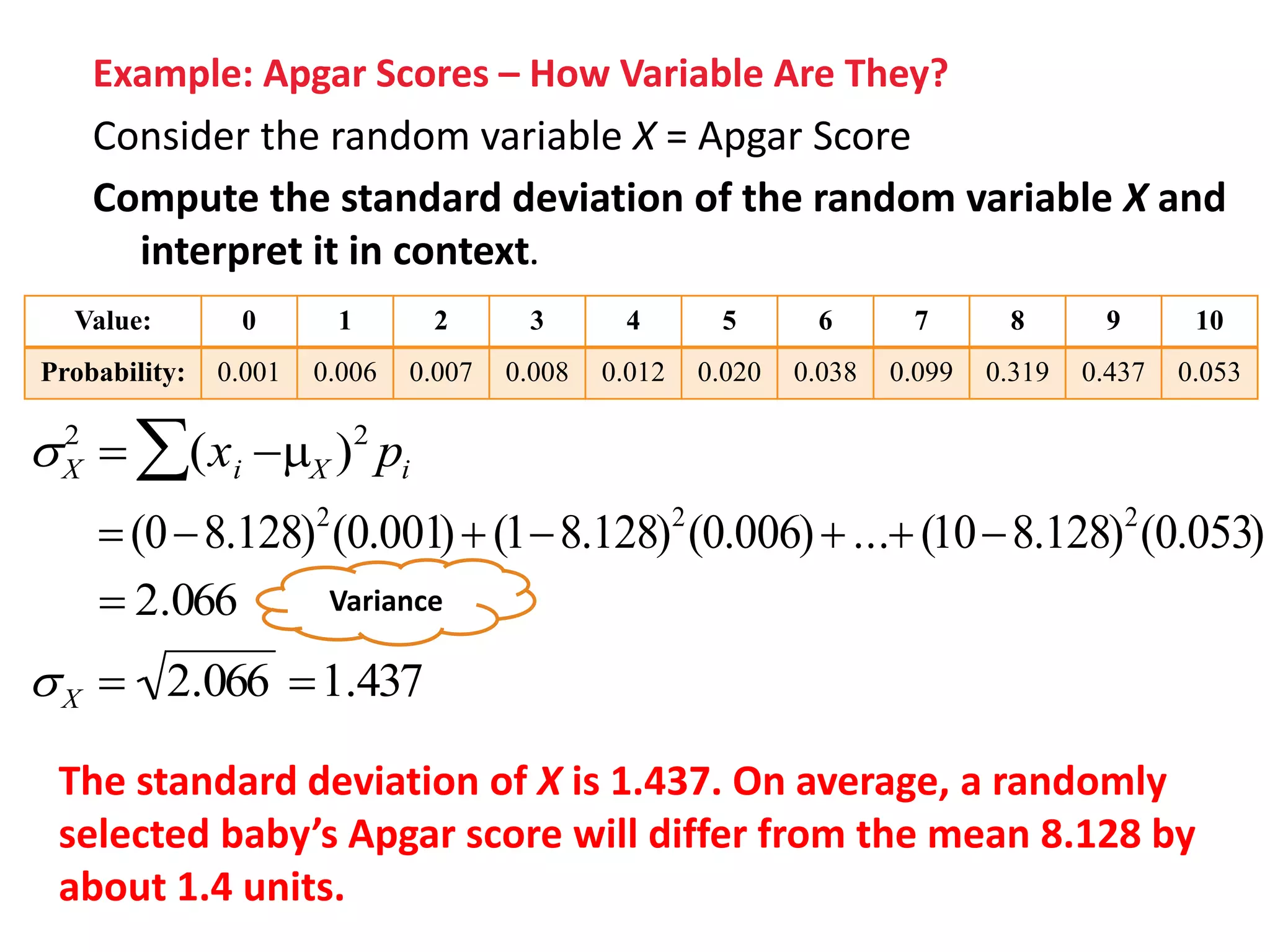
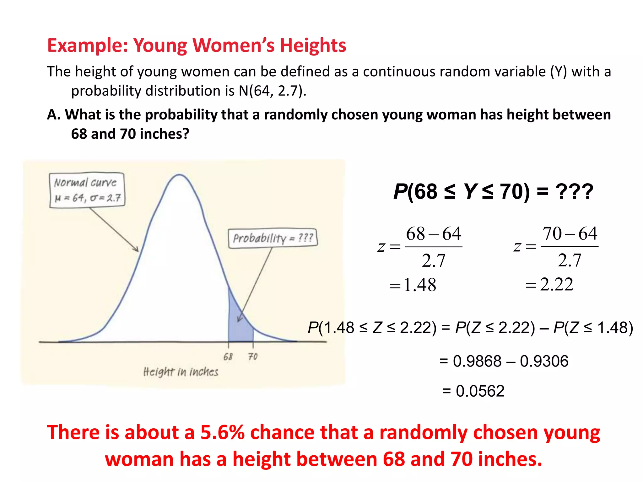
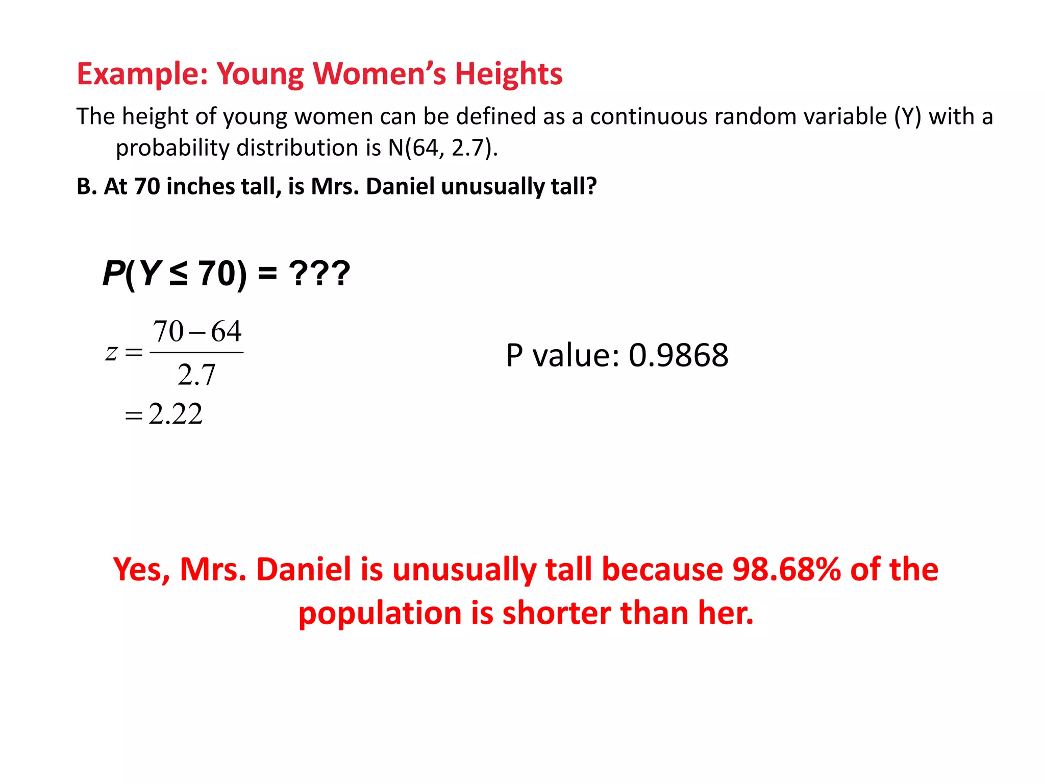
The document discusses discrete and continuous random variables. It defines discrete random variables as variables that can take on countable values, like the number of heads from coin flips. Continuous random variables can take any value within a range, like height. The document explains how to calculate and interpret the mean, standard deviation, and probabilities of events for both types of random variables using examples like Apgar scores for babies and heights of young women.

1. 6.1:
Discrete and Continuous
Random Variables

2. Section 6.1
Discrete & Continuous Random Variables
After this section, you should be able to…
APPLY the concept of discrete random variables to a
variety of statistical settings
CALCULATE and INTERPRET the mean (expected value) of
a discrete random variable
CALCULATE and INTERPRET the standard deviation (and
variance) of a discrete random variable
DESCRIBE continuous random variables

3. Random
Variables
• A random variable, usually
written as X, is a variable
whose possible values are
numerical outcomes of a
random phenomenon.
• There are two types of
random variables, discrete
random variables and
continuous random
variables.

4. Discrete Random Variables
• A discrete random variable is one which may take on
only a countable number of distinct values such as 0,
1, 2, 3, 4,....
• Discrete random variables are usually (but not
necessarily) counts.
• Examples:
• number of children in a family
• the Friday night attendance at a cinema
• the number of patients a doctor sees in one day
• the number of defective light bulbs in a box of ten
• the number of “heads” flipped in 3 trials

5. Consider tossing a fair coin 3 times.
Define X = the number of heads obtained
X = 0: TTT
X = 1: HTT THT TTH
X = 2: HHT HTH THH
X = 3: HHH
Value 0 1 2 3
Probability 1/8 3/8 3/8 1/8
The probability distribution of a discrete random variable is
a list of probabilities associated with each of its possible
values
Probability Distribution

6. If you roll a pair of dice and record the sum for each trial, after
an infinite number of times, your distribution will approximate
the probability distribution on the next slide.
Rolling Dice: Probability
Distribution

8. Discrete Random Variables
A discrete random variable X takes a fixed set of possible
values with gaps between. The probability distribution of
a discrete random variable X lists the values xi and their
probabilities pi:
Value: x1 x2 x3 …
Probability: p1 p2 p3 …
The probabilities pi must satisfy two requirements:
1. Every probability pi is a number between 0 and 1.
2. The sum of the probabilities is 1.
To find the probability of any event, add the probabilities pi
of the particular values xi that make up the event.

9. Describing the (Probability) Distribution
When analyzing discrete random variables, we’ll follow the
same strategy we used with quantitative data – describe the
shape, center (mean), and spread (standard deviation), and
identify any outliers.

10. Example: Babies’ Health at Birth
Background details are on page 343.
(a)Show that the probability distribution for X is legitimate.
(b)Make a histogram of the probability distribution. Describe
what you see.
(c)Apgar scores of 7 or higher indicate a healthy baby. What is
P(X ≥ 7)?
Value: 0 1 2 3 4 5 6 7 8 9 10
Probability: 0.001 0.006 0.007 0.008 0.012 0.020 0.038 0.099 0.319 0.437 0.053

11. Example: Babies’ Health at Birth
Background details are on page 343.
(a)Show that the probability distribution for X is legitimate.
(b)Make a histogram of the probability distribution. Describe
the distribution.
(c)Apgar scores of 7 or higher indicate a healthy baby. What is
P(X ≥ 7)?
(a) All probabilities are between 0 and 1 and the probabilities
sum to 1. This is a legitimate probability distribution.
Value: 0 1 2 3 4 5 6 7 8 9 10
Probability: 0.001 0.006 0.007 0.008 0.012 0.020 0.038 0.099 0.319 0.437 0.053

12. Example: Babies’ Health at Birth
b. Make a histogram of the probability distribution. Describe what you see.
c. Apgar scores of 7 or higher indicate a healthy baby. What is P(X ≥ 7)?
(b) The left-skewed shape of the distribution suggests a randomly
selected newborn will have an Apgar score at the high end of the scale.
While the range is from 0 to 10, there is a VERY small chance of getting
a baby with a score of 5 or lower. There are no obvious outliers. The
center of the distribution is approximately 8.
(c) P(X ≥ 7) = .908
We’d have a 91 % chance
of randomly choosing a
healthy baby.
Value: 0 1 2 3 4 5 6 7 8 9 10
Probability: 0.001 0.006 0.007 0.008 0.012 0.020 0.038 0.099 0.319 0.437 0.053

13. Mean of a Discrete Random Variable
The mean of any discrete random variable is an average of
the possible outcomes, with each outcome weighted by its
probability.
Suppose that X is a discrete random variable whose
probability distribution is
Value: x1 x2 x3 …
Probability: p1 p2 p3 …
To find the mean (expected value) of X, multiply each
possible value by its probability, then add all the products:
x  E(X)  x1p1  x2 p2  x3 p3  ...
 xi pi

14. Example: Apgar Scores – What’s Typical?
Consider the random variable X = Apgar Score
Compute the mean of the random variable X and interpret it in context.
Value: 0 1 2 3 4 5 6 7 8 9 10
Probability: 0.001 0.006 0.007 0.008 0.012 0.020 0.038 0.099 0.319 0.437 0.053

x  E(X)  xi pi

15. Example: Apgar Scores – What’s Typical?
Consider the random variable X = Apgar Score
Compute the mean of the random variable X and interpret it in context.
Value: 0 1 2 3 4 5 6 7 8 9 10
Probability: 0.001 0.006 0.007 0.008 0.012 0.020 0.038 0.099 0.319 0.437 0.053
x  E(X)  xi pi

(0)(0.001)(1)(0.006)(2)(0.007)...(10)(0.053)

 8.128
The mean Apgar score of a randomly selected newborn is 8.128.
This is the long-term average Agar score of many, many
randomly chosen babies.
Note: The expected value does not need to be a possible value of
X or an integer! It is a long-term average over many repetitions.

16. Standard Deviation of a Discrete
Random Variable
The definition of the variance of a random variable is similar to
the definition of the variance for a set of quantitative data. To
get the standard deviation of a random variable, take the square
root of the variance.
Suppose that X is a discrete random variable whose
probability distribution is
Value: x1 x2 x3 …
Probability: p1 p2 p3 …
and that µX is the mean of X. The variance of X is
Var(X)  X
2
 (x1 X )2
p1  (x2 X )2
p2  (x3 X )2
p3  ...
 (xi X )2
pi

17. Example: Apgar Scores – How Variable Are They?
Consider the random variable X = Apgar Score
Compute the standard deviation of the random variable X and
interpret it in context.
Value: 0 1 2 3 4 5 6 7 8 9 10
Probability: 0.001 0.006 0.007 0.008 0.012 0.020 0.038 0.099 0.319 0.437 0.053
X
2
 (xi X )2
pi
(08.128)2
(0.001)(18.128)2
(0.006)...(108.128)2
(0.053)
 2.066
The standard deviation of X is 1.437. On average, a randomly
selected baby’s Apgar score will differ from the mean 8.128 by
about 1.4 units.
X  2.066 1.437
Variance

18. Continuous Random Variable
• A continuous random variable is one which
takes an infinite number of possible values.
• Continuous random variables are usually
measurements.
• Examples:
– height
– weight
– the amount of sugar in an orange
– the time required to run a mile.

19. Continuous Random Variables
A continuous random variable X takes on all values in an
interval of numbers. The probability distribution of X is
described by a density curve. The probability of any
event is the area under the density curve and above the
values of X that make up the event.

20. • A continuous random variable is
not defined at specific values.
• Instead, it is defined over an
interval of value; however, you
can calculate the probability of a
range of values.
• It is very similar to z-scores and
normal distribution calculations.
Continuous Random Variables

21. Example: Young Women’s Heights
The height of young women can be defined as a continuous
random variable (Y) with a probability distribution is N(64,
2.7).
A. What is the probability that a randomly chosen young
woman has height between 68 and 70 inches?
P(68 ≤ Y ≤ 70) = ???

22. Example: Young Women’s Heights
The height of young women can be defined as a continuous random variable (Y) with a
probability distribution is N(64, 2.7).
A. What is the probability that a randomly chosen young woman has height between
68 and 70 inches?
P(68 ≤ Y ≤ 70) = ???

z 
6864
2.7
1.48

z 
7064
2.7
 2.22
P(1.48 ≤ Z ≤ 2.22) = P(Z ≤ 2.22) – P(Z ≤ 1.48)
= 0.9868 – 0.9306
= 0.0562
There is about a 5.6% chance that a randomly chosen young
woman has a height between 68 and 70 inches.

23. Example: Young Women’s Heights
The height of young women can be defined as a continuous
random variable (Y) with a probability distribution is N(64,
2.7).
B. At 70 inches tall, is Mrs. Daniel unusually tall?

24. Example: Young Women’s Heights
The height of young women can be defined as a continuous random variable (Y) with a
probability distribution is N(64, 2.7).
B. At 70 inches tall, is Mrs. Daniel unusually tall?
P(Y ≤ 70) = ???

z 
7064
2.7
 2.22
P value: 0.9868
Yes, Mrs. Daniel is unusually tall because 98.68% of the
population is shorter than her.