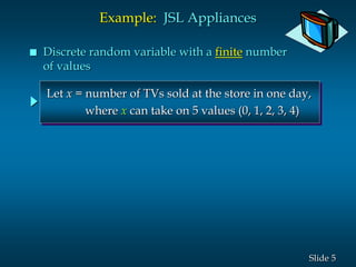
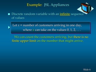
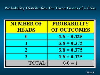
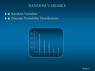
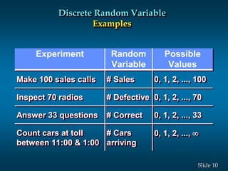
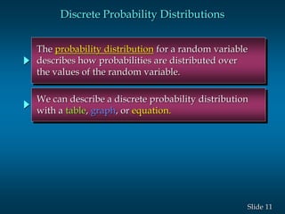
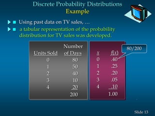
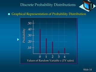
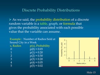
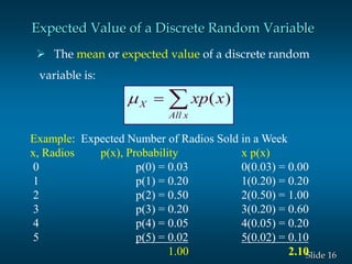
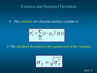
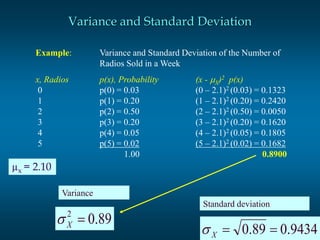
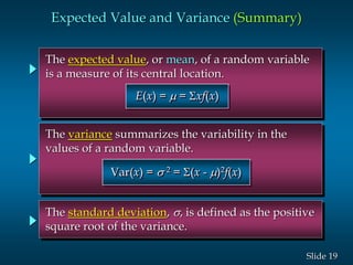
The document discusses random variables and probability distributions. It provides examples of random variables like the number of heads from tossing a coin 3 times. The possible values and probabilities are shown in tables and graphs. Key concepts explained include the expected value (mean) of a random variable being the sum of each value multiplied by its probability. The variance is the sum of the squared differences between each value and the mean, and measures variability. The standard deviation is the square root of the variance.

1. 1Slide
Random Variables
Definition & Example
 Definition: A random variable is a quantity resulting from a
random experiment that, by chance, can assume different values.
 Example: Consider a random experiment in which a coin is
tossed three times. Let X be the number of heads. Let H
represent the outcome of a head and T the outcome of a tail.

2. 2Slide
 The sample space for such an experiment will be: TTT, TTH,
THT, THH, HTT, HTH, HHT, HHH.
 Thus the possible values of X (number of heads) are X = 0, 1, 2,
3.
 This association is shown in the next slide.
 Note: In this experiment, there are 8 possible outcomes in the
sample space. Since they are all equally likely to occur, each
outcome has a probability of 1/8 of occurring.
Example (Continued)

3. 3Slide
TTT
TTH
THT
THH
HTT
HTH
HHT
HHH
0
1
1
2
1
2
2
3
Sample
Space
X
Example (Continued)

4. 4Slide
 The outcome of zero heads occurred only once.
 The outcome of one head occurred three times.
 The outcome of two heads occurred three times.
 The outcome of three heads occurred only once.
 From the definition of a random variable, X as defined in
this experiment, is a random variable.
 X values are determined by the outcomes of the experiment.
Example (Continued)

5. 5Slide
Let x = number of TVs sold at the store in one day,
where x can take on 5 values (0, 1, 2, 3, 4)
Example: JSL Appliances
 Discrete random variable with a finite number
of values

6. 6Slide
Let x = number of customers arriving in one day,
where x can take on the values 0, 1, 2, . . .
Example: JSL Appliances
 Discrete random variable with an infinite sequence
of values
We can count the customers arriving, but there is no
finite upper limit on the number that might arrive.

7. 7Slide
Probability Distribution: Definition
 Definition: A probability distribution is a listing of all the
outcomes of an experiment and their associated probabilities.
 The probability distribution for the random variable X
(number of heads) in tossing a coin three times is shown next.

8. 8Slide
Probability Distribution for Three Tosses of a Coin

9. 9Slide
RANDOM VARIABLE
.10
.20
.30
.40
0 1 2 3 4
 Random Variables
 Discrete Probability Distributions

10. 10Slide
Discrete Random Variable
Examples
Experiment Random
Variable
Possible
Values
Make 100 sales calls # Sales 0, 1, 2, ..., 100
Inspect 70 radios # Defective 0, 1, 2, ..., 70
Answer 33 questions # Correct 0, 1, 2, ..., 33
Count cars at toll
between 11:00 & 1:00
# Cars
arriving
0, 1, 2, ..., 

11. 11Slide
The probability distribution for a random variable
describes how probabilities are distributed over
the values of the random variable.
We can describe a discrete probability distribution
with a table, graph, or equation.
Discrete Probability Distributions

12. 12Slide
The probability distribution is defined by a
probability function, denoted by f(x), which provides
the probability for each value of the random variable.
The required conditions for a discrete probability
function are:
Discrete Probability Distributions
f(x) > 0
f(x) = 1
P(X) ≥ 0
ΣP(X) = 1

13. 13Slide
 a tabular representation of the probability
distribution for TV sales was developed.
 Using past data on TV sales, …
Number
Units Sold of Days
0 80
1 50
2 40
3 10
4 20
200
x f(x)
0 .40
1 .25
2 .20
3 .05
4 .10
1.00
80/200
Discrete Probability Distributions
Example

14. 14Slide
.10
.20
.30
.40
.50
0 1 2 3 4
Values of Random Variable x (TV sales)
Probability
Discrete Probability Distributions
 Graphical Representation of Probability Distribution

15. 15Slide
Discrete Probability Distributions
 As we said, the probability distribution of a discrete
random variable is a table, graph, or formula that
gives the probability associated with each possible
value that the variable can assume.
Example : Number of Radios Sold at
Sound City in a Week
x, Radios p(x), Probability
0 p(0) = 0.03
1 p(1) = 0.20
2 p(2) = 0.50
3 p(3) = 0.20
4 p(4) = 0.05
5 p(5) = 0.02

16. 16Slide
Expected Value of a Discrete Random Variable
 The mean or expected value of a discrete random
variable is:

xAll
X xxp )(
Example: Expected Number of Radios Sold in a Week
x, Radios p(x), Probability x p(x)
0 p(0) = 0.03 0(0.03) = 0.00
1 p(1) = 0.20 1(0.20) = 0.20
2 p(2) = 0.50 2(0.50) = 1.00
3 p(3) = 0.20 3(0.20) = 0.60
4 p(4) = 0.05 4(0.05) = 0.20
5 p(5) = 0.02 5(0.02) = 0.10
1.00 2.10

17. 17Slide
Variance and Standard Deviation
 The variance of a discrete random variable is:
 
xAll
XX xpx )()( 22

2
XX  
 The standard deviation is the square root of the variance.

18. 18Slide
Example: Variance and Standard Deviation of the Number of
Radios Sold in a Week
x, Radios p(x), Probability (x - X)2 p(x)
0 p(0) = 0.03 (0 – 2.1)2 (0.03) = 0.1323
1 p(1) = 0.20 (1 – 2.1)2 (0.20) = 0.2420
2 p(2) = 0.50 (2 – 2.1)2 (0.50) = 0.0050
3 p(3) = 0.20 (3 – 2.1)2 (0.20) = 0.1620
4 p(4) = 0.05 (4 – 2.1)2 (0.05) = 0.1805
5 p(5) = 0.02 (5 – 2.1)2 (0.02) = 0.1682
1.00 0.8900
89.02
X
Variance
9434.089.0 X
Standard deviation
Variance and Standard Deviation
µx = 2.10

19. 19Slide
Expected Value and Variance (Summary)
The expected value, or mean, of a random variable
is a measure of its central location.
The variance summarizes the variability in the
values of a random variable.
The standard deviation, , is defined as the positive
square root of the variance.
Var(x) =  2 = (x - )2f(x)
E(x) =  = xf(x)