1. The document discusses different types of probability distributions including discrete, continuous, binomial, Poisson, and normal distributions.
2. It provides examples of how to calculate probabilities and expected values for each distribution using concepts like probability density functions, mean, standard deviation, and combinations.
3. Key differences between distributions are highlighted such as discrete probabilities being determined by areas under a curve for continuous distributions and Poisson distribution approximating binomial for large numbers of trials.
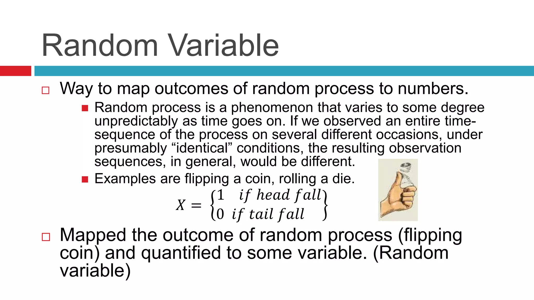
Overview of probability distribution and random variables, including mapping outcomes of random processes.
Explains discrete and continuous random variables with examples; discrete variables have distinct values, continuous variables can take on any value in an interval.
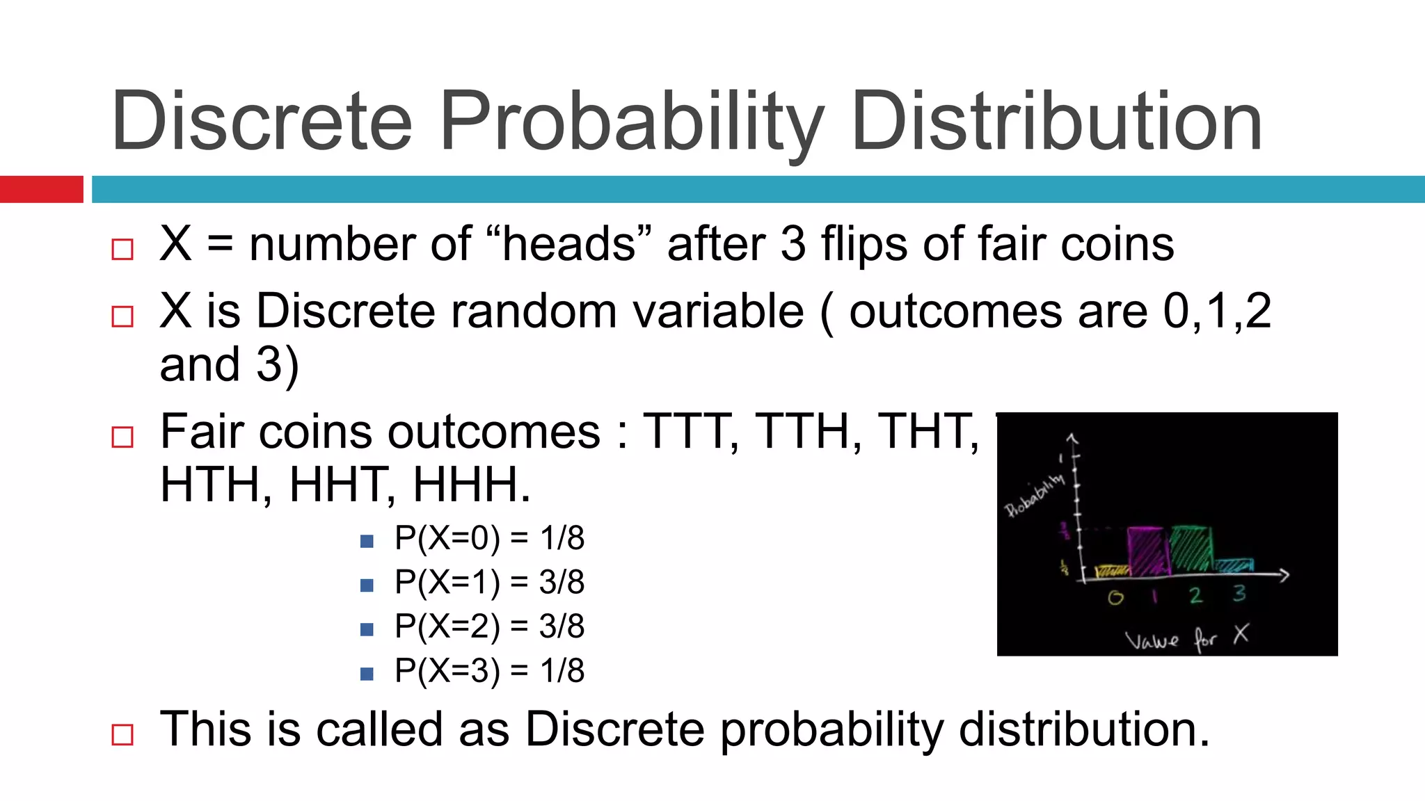
Details on discrete probability distribution, exemplified by coin flips, with calculated probabilities for outcomes 0 to 3 heads.
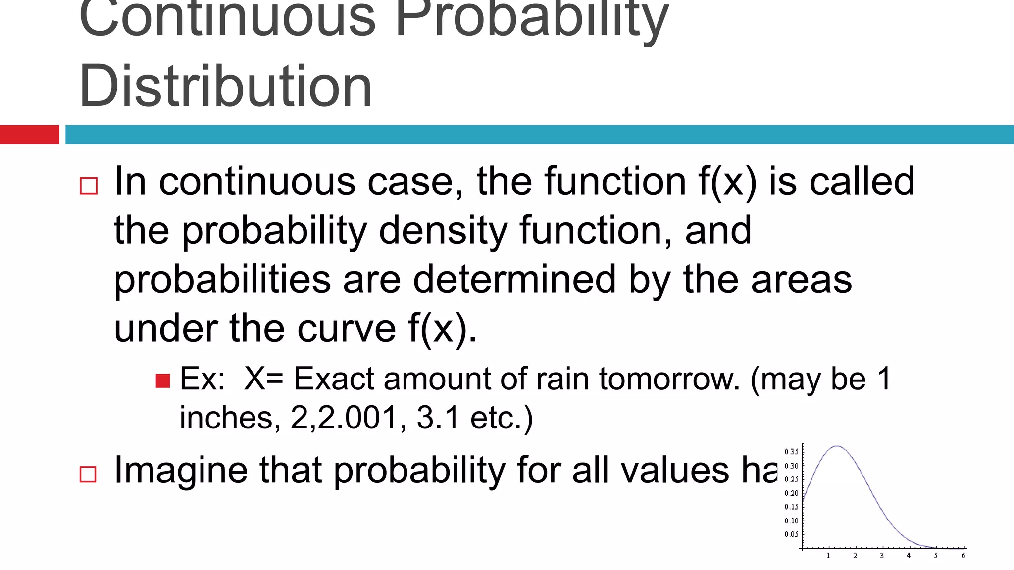
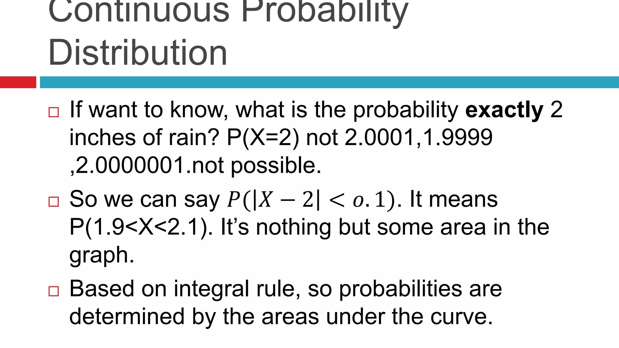
Introduces probability density functions for continuous variables and explains probability determination through area under curves.
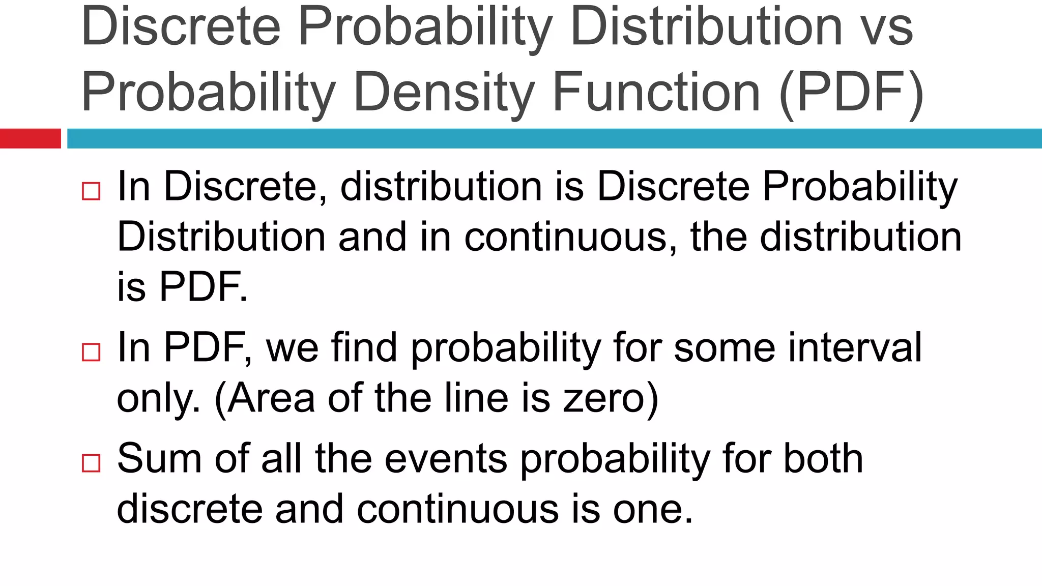
Differences between discrete probability distributions and PDFs, emphasizing sum of probabilities equaling one.
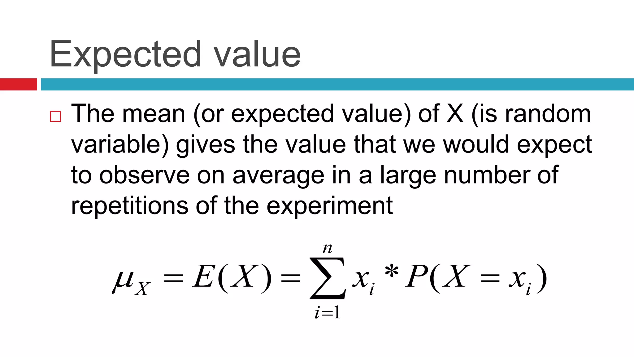
Definition of expected value as the mean of random variables calculated over numerous trials.
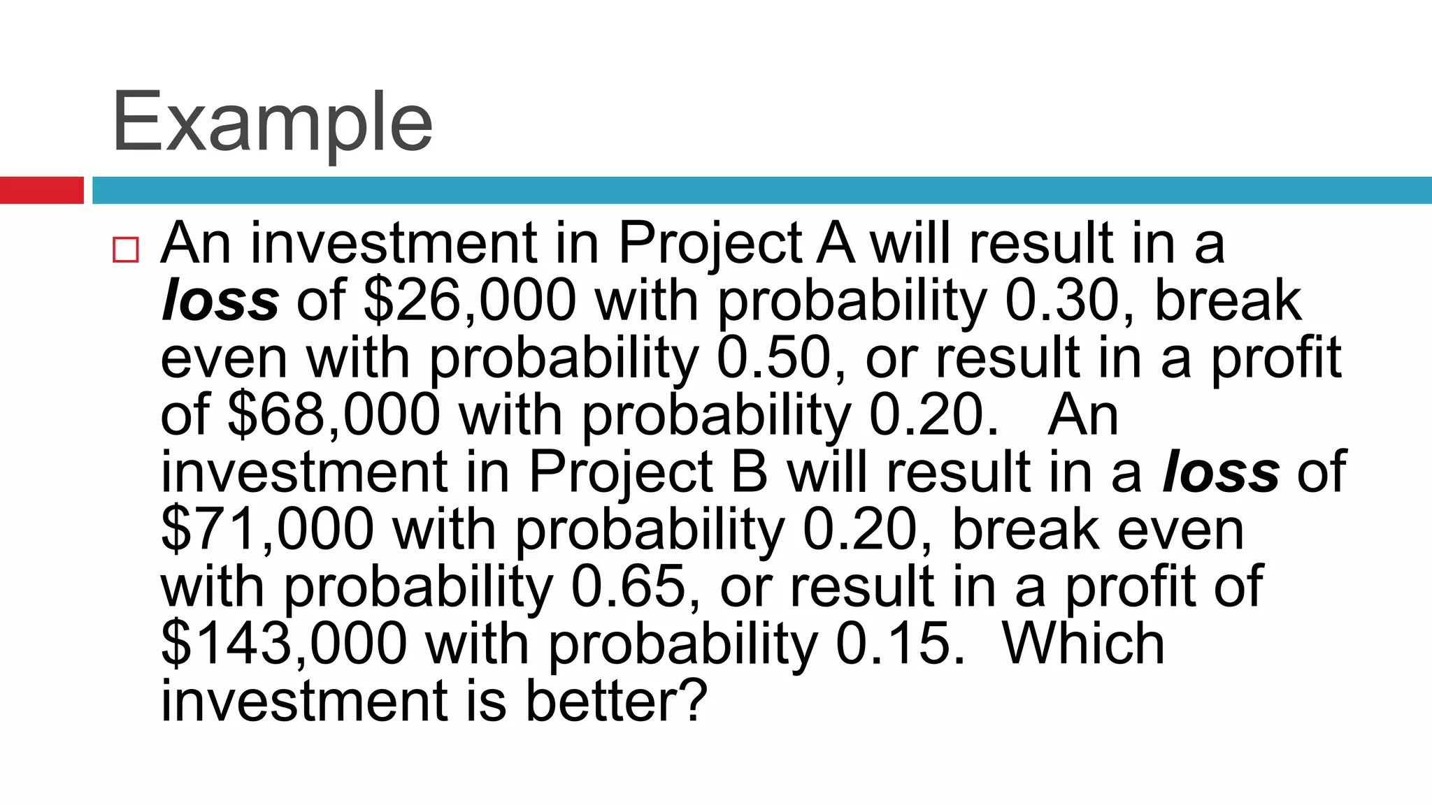
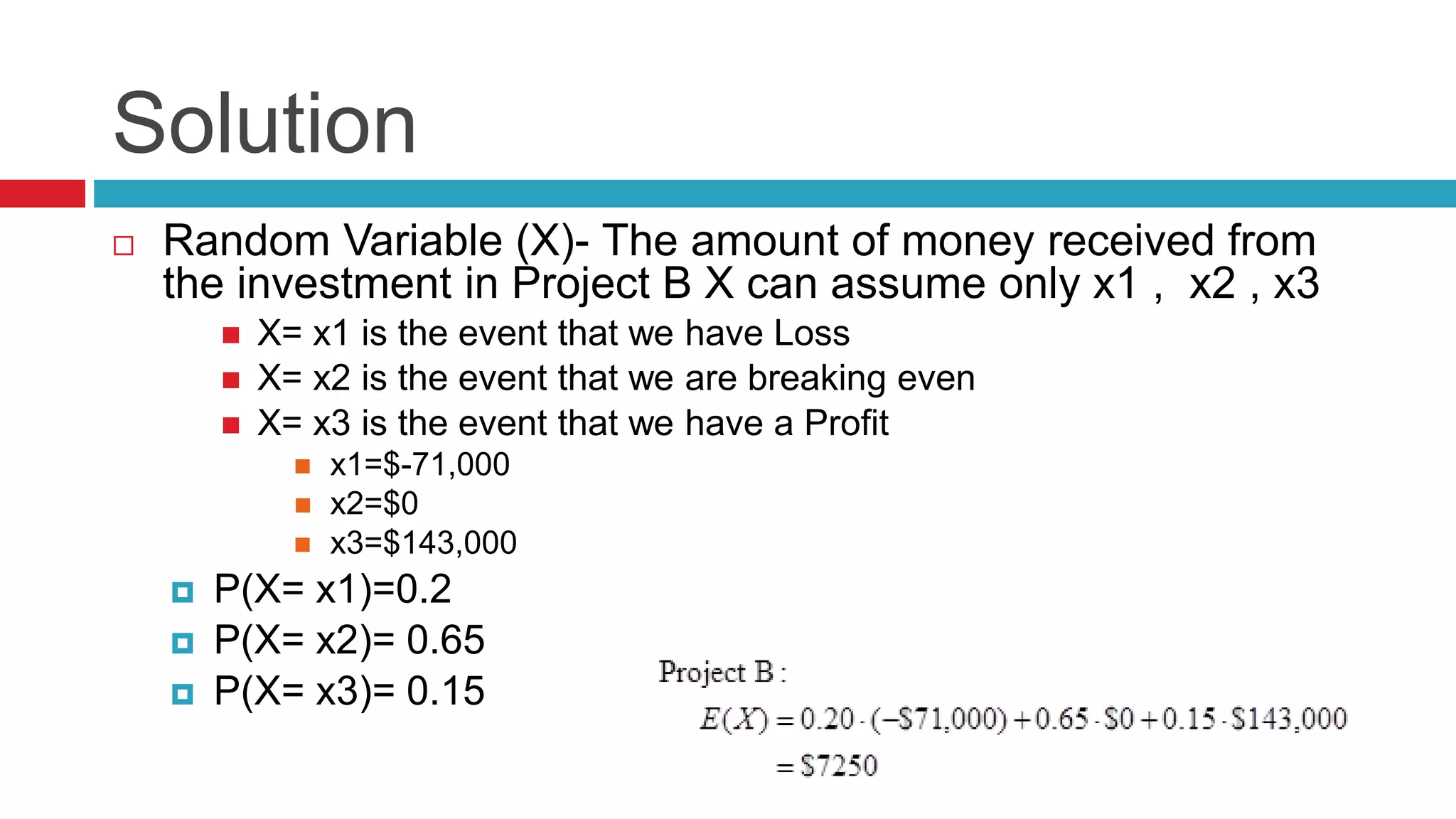
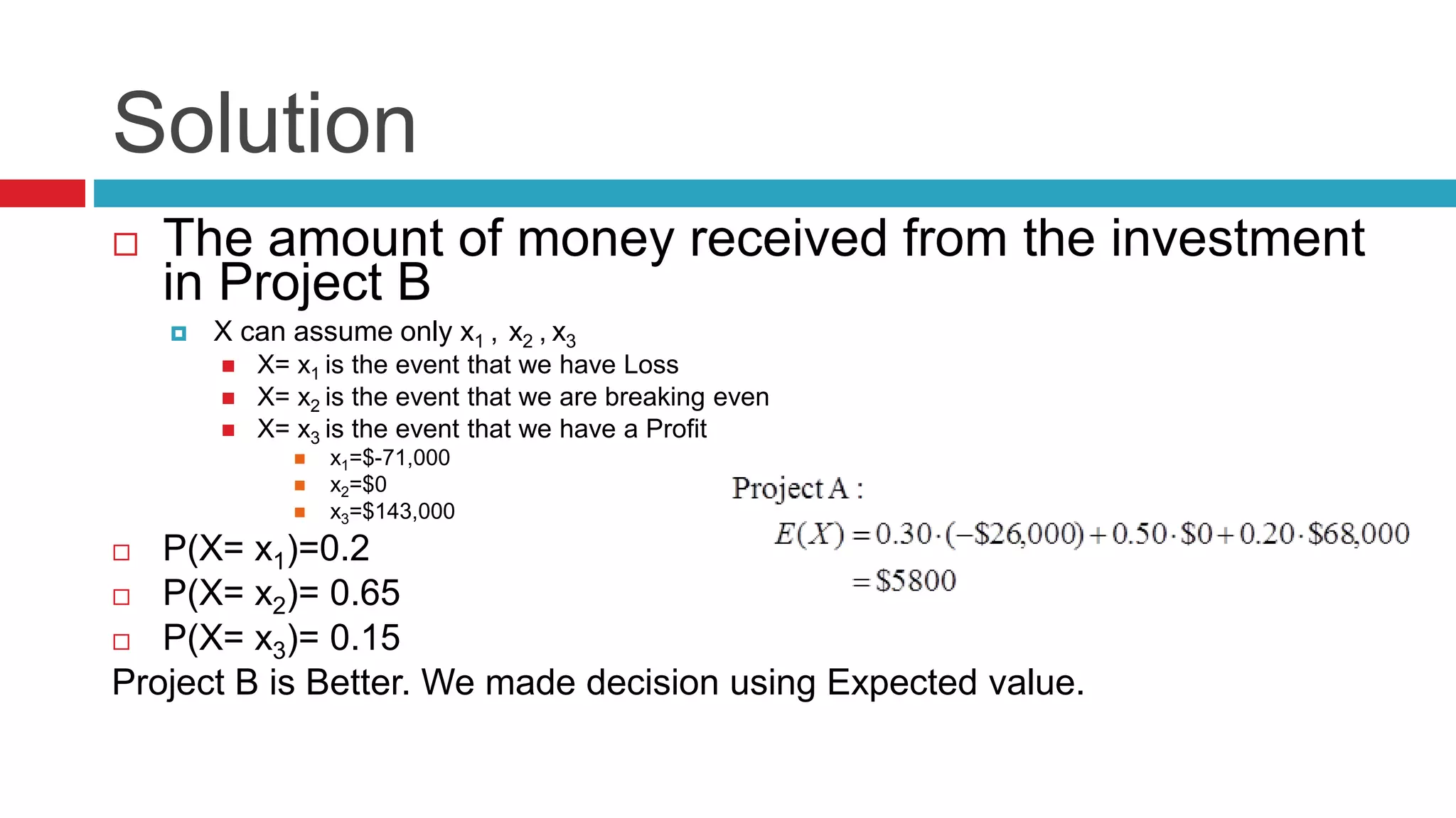
Compares investments in Projects A and B through expected value analysis to decide which is better.
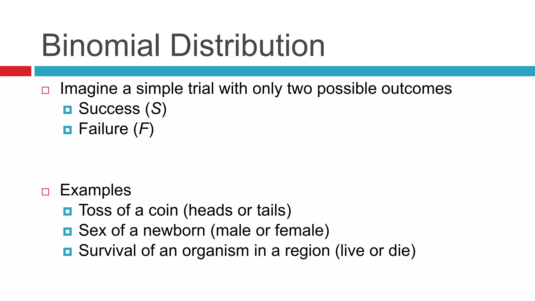
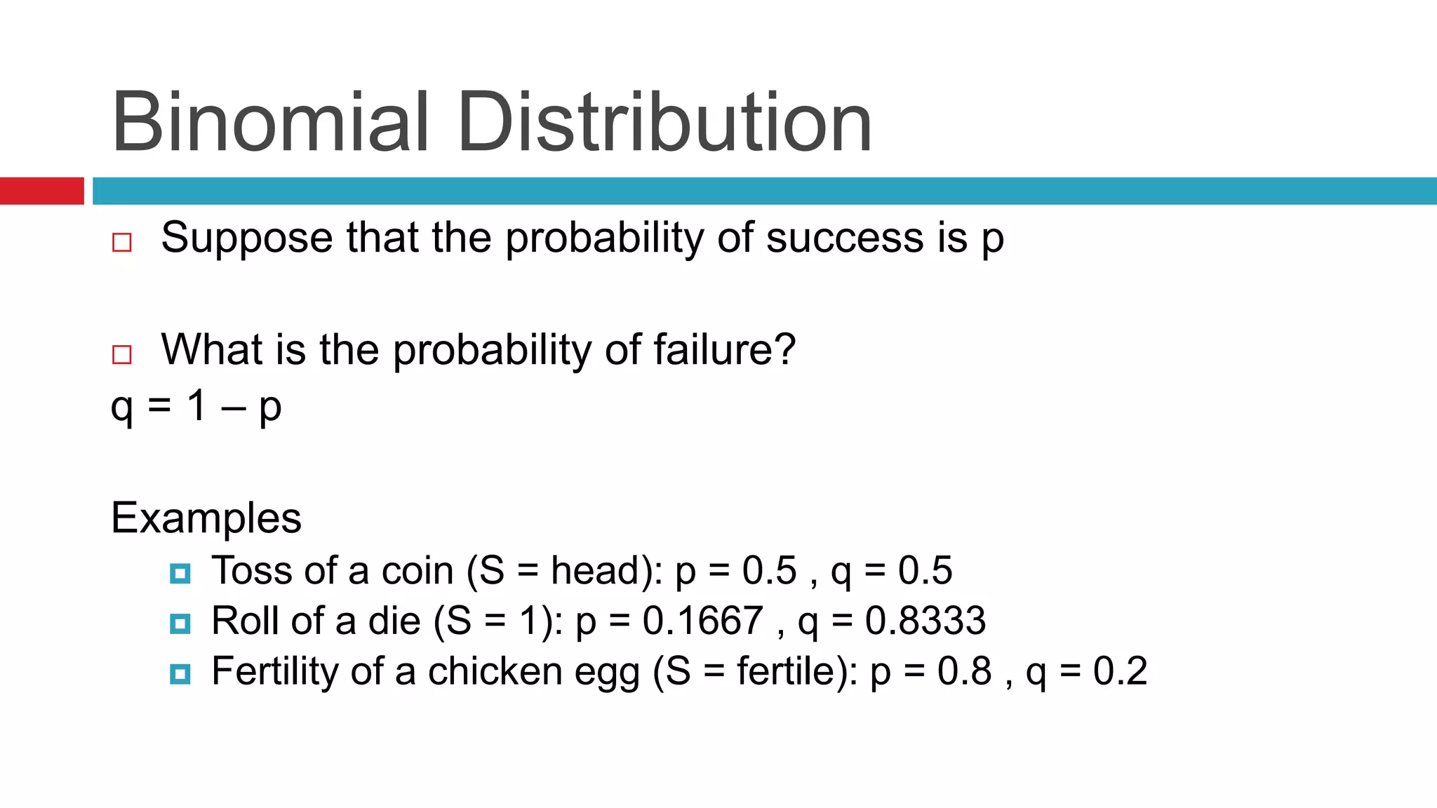
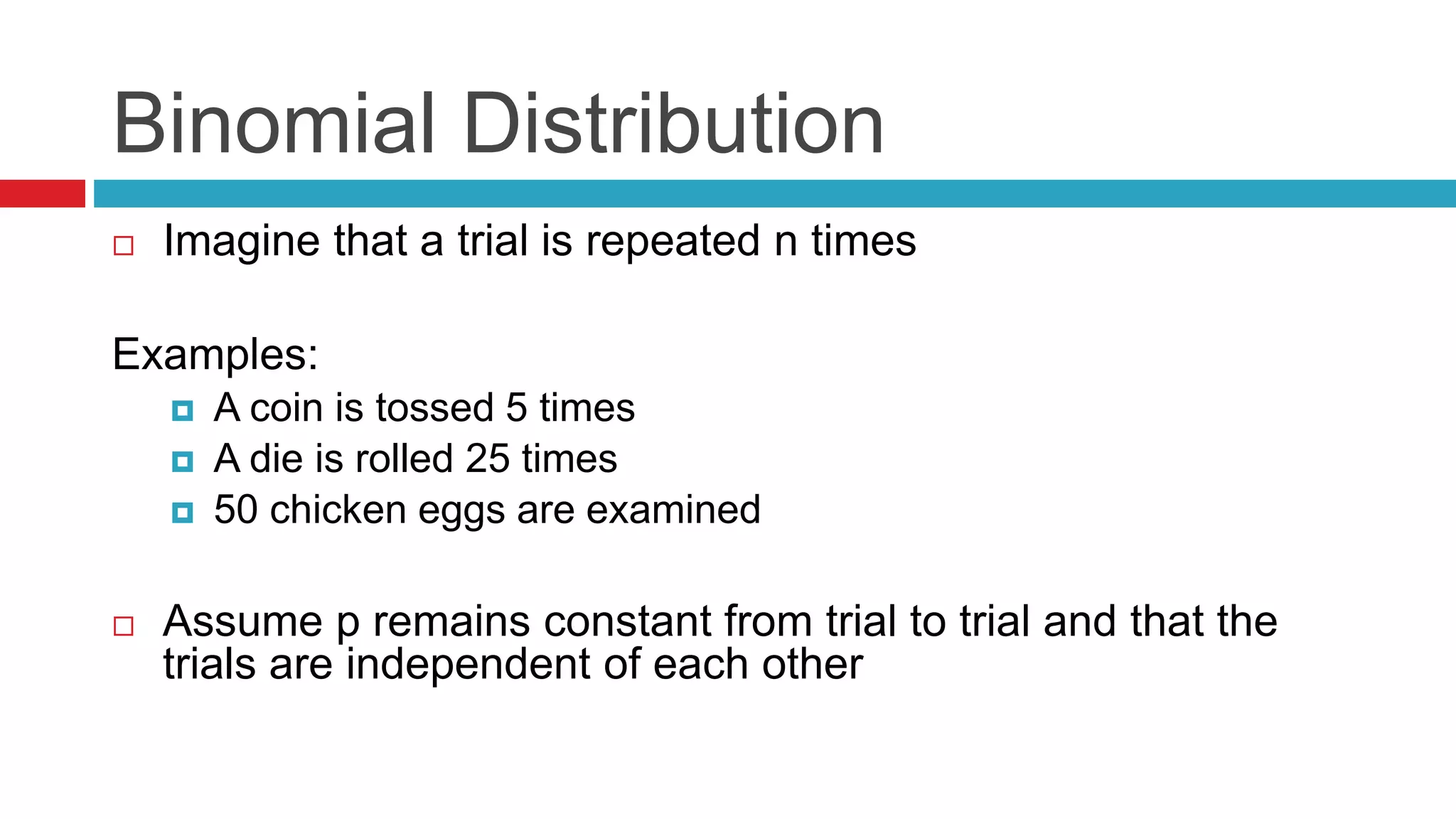
Introduces binomial distribution with trials yielding two outcomes and gives examples of success and failure scenarios.
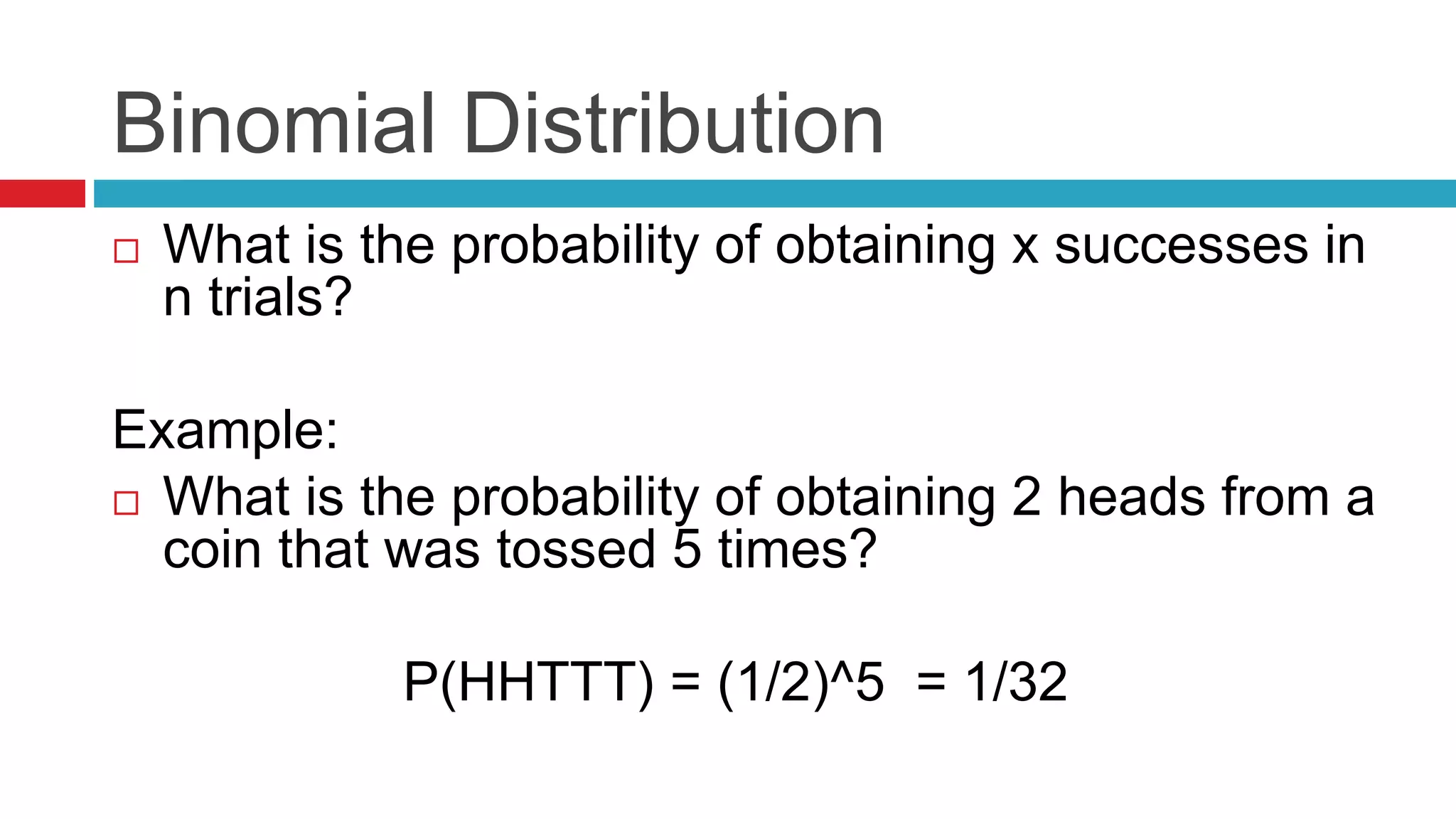
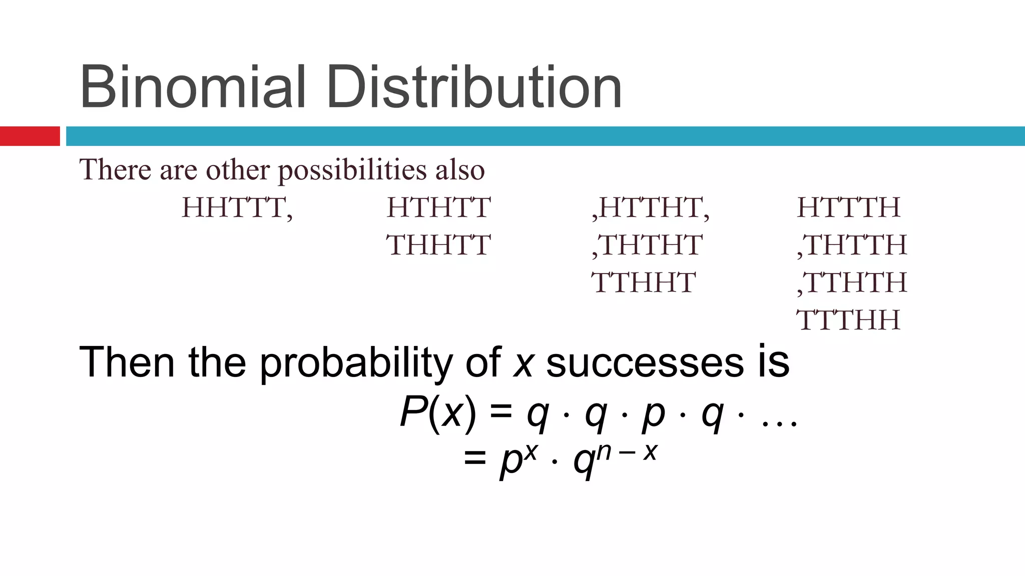
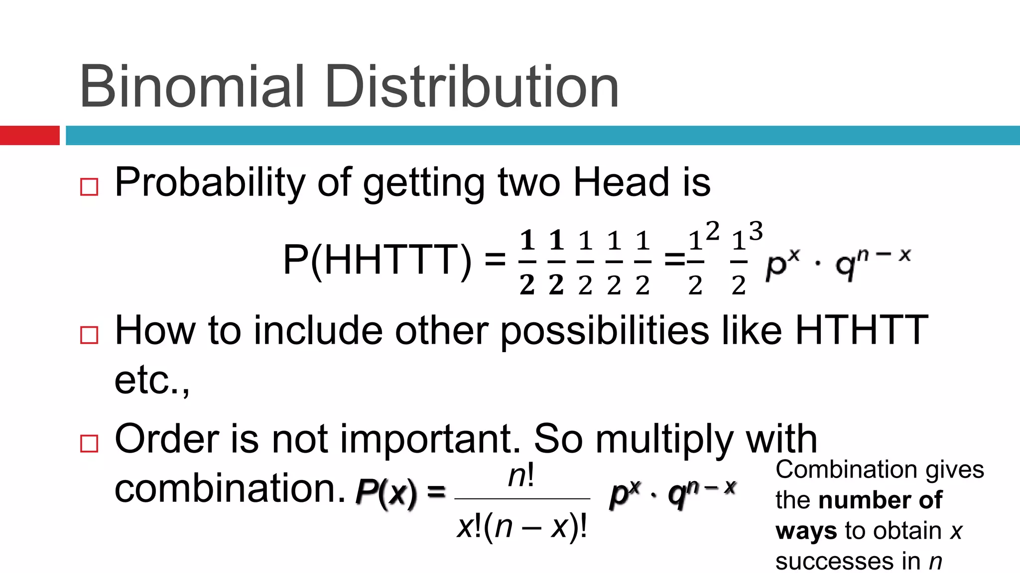
Techniques to calculate probabilities of successes in binomial distribution scenarios, utilizing combinations.
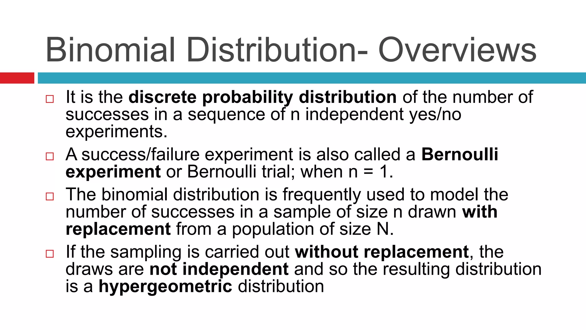
Describes binomial distribution's application in independent experiments and compares to hypergeometric distribution.
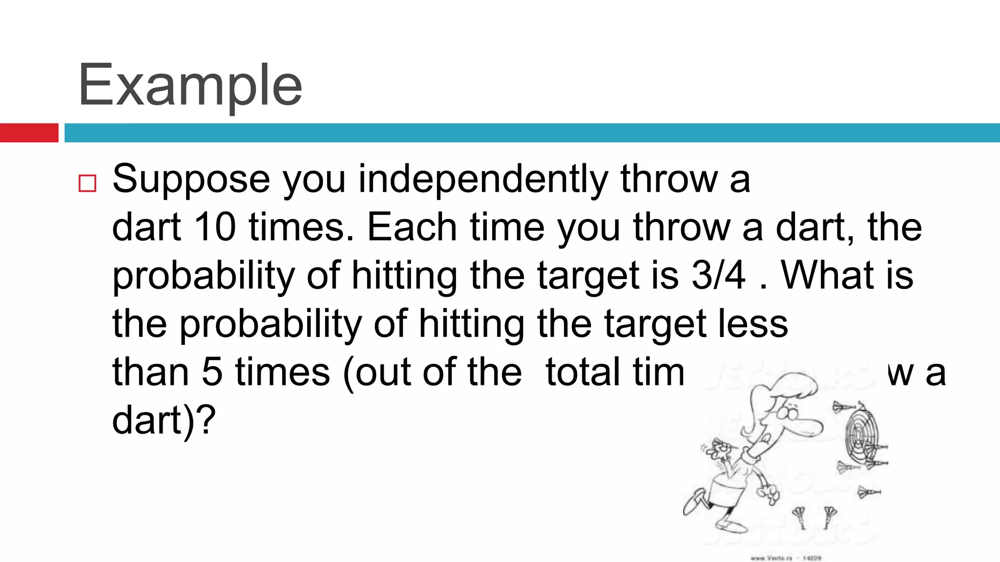
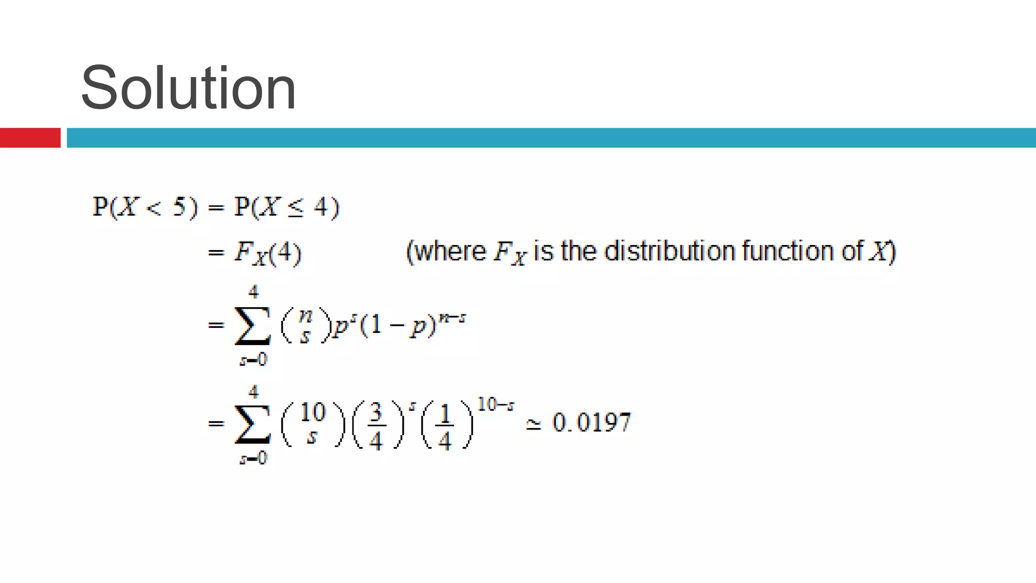
Calculates probability of hitting a dart target using binomial distribution concept.
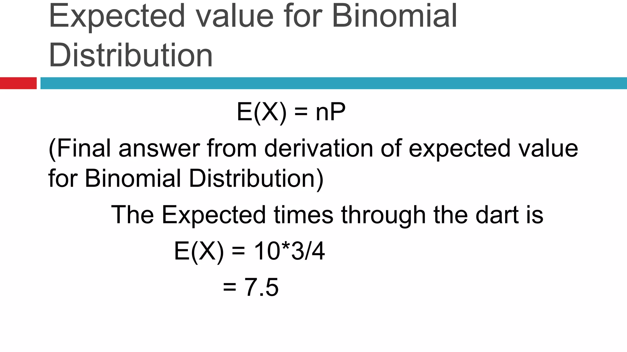
Derives expected value formula for binomial distribution, demonstrating calculation with given probability.
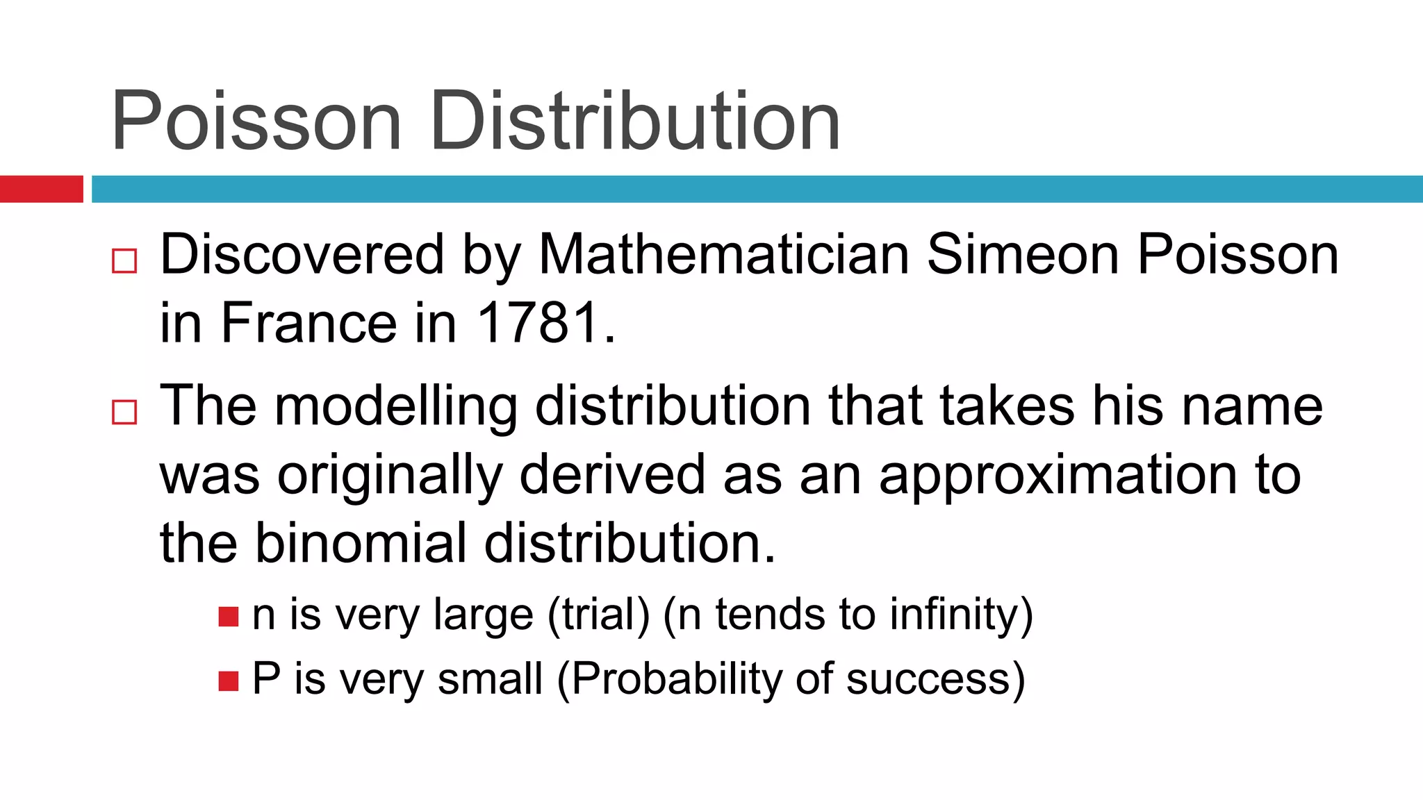
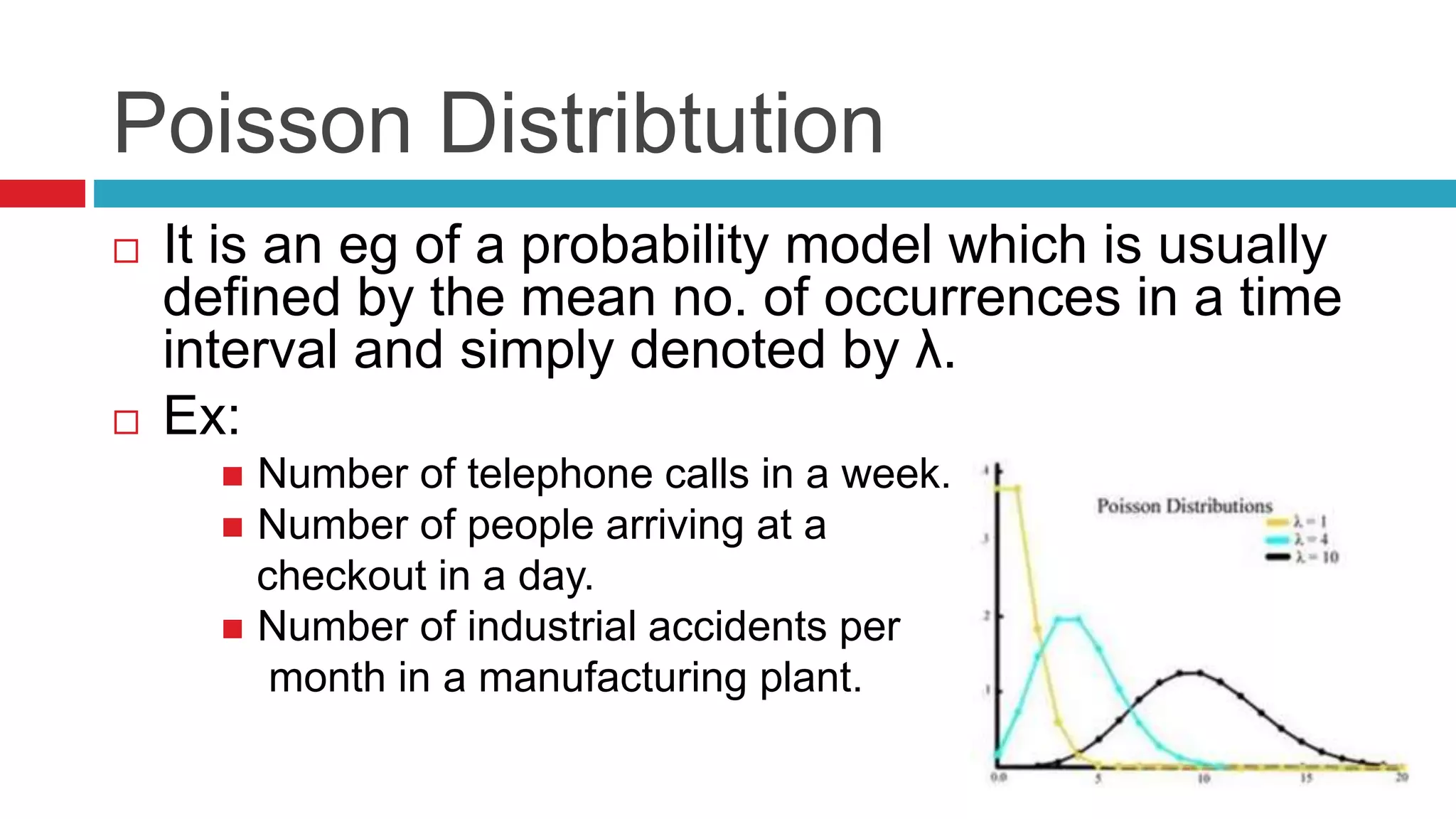
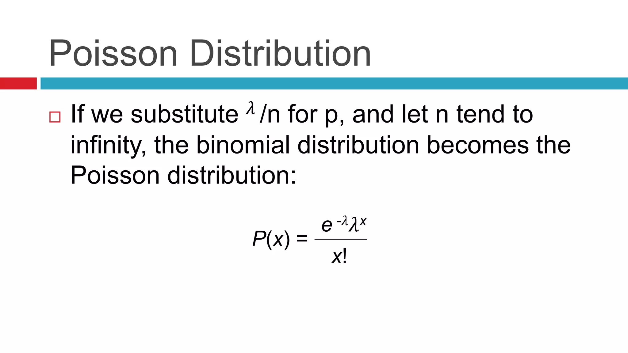
Overview of Poisson distribution and its origins as an approximation of binomial distribution in certain conditions.
Criteria for applying the Poisson distribution including independence and constancy of occurrence probabilities.
Shows derivation of Poisson distribution formula in relation to binomial distribution.
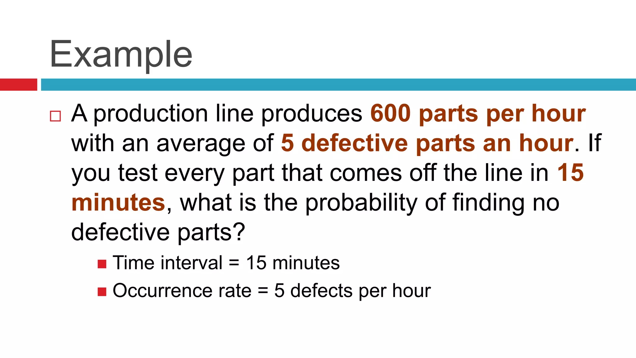
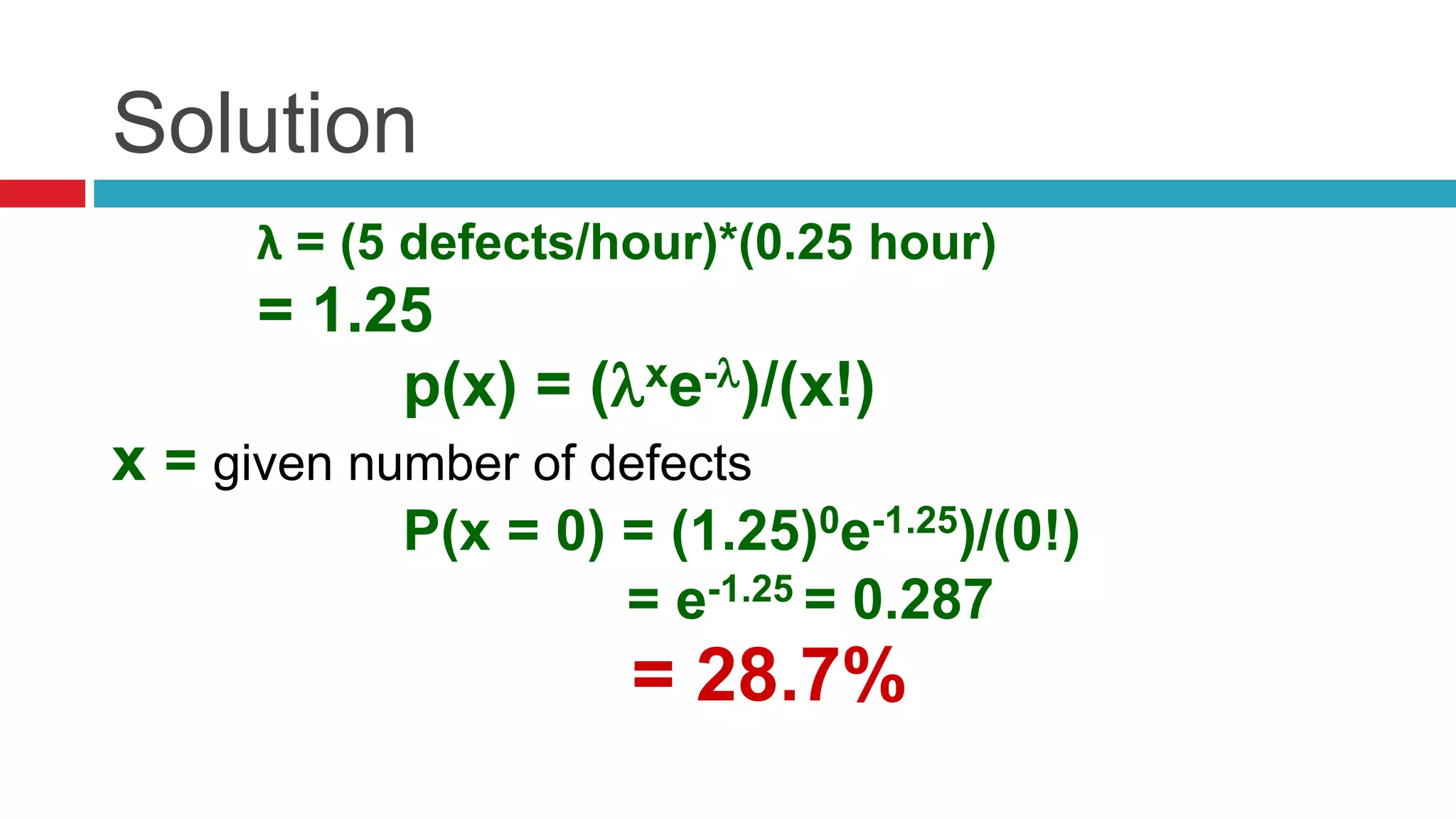
Calculates the probability of finding no defective parts from a production line using Poisson probability.
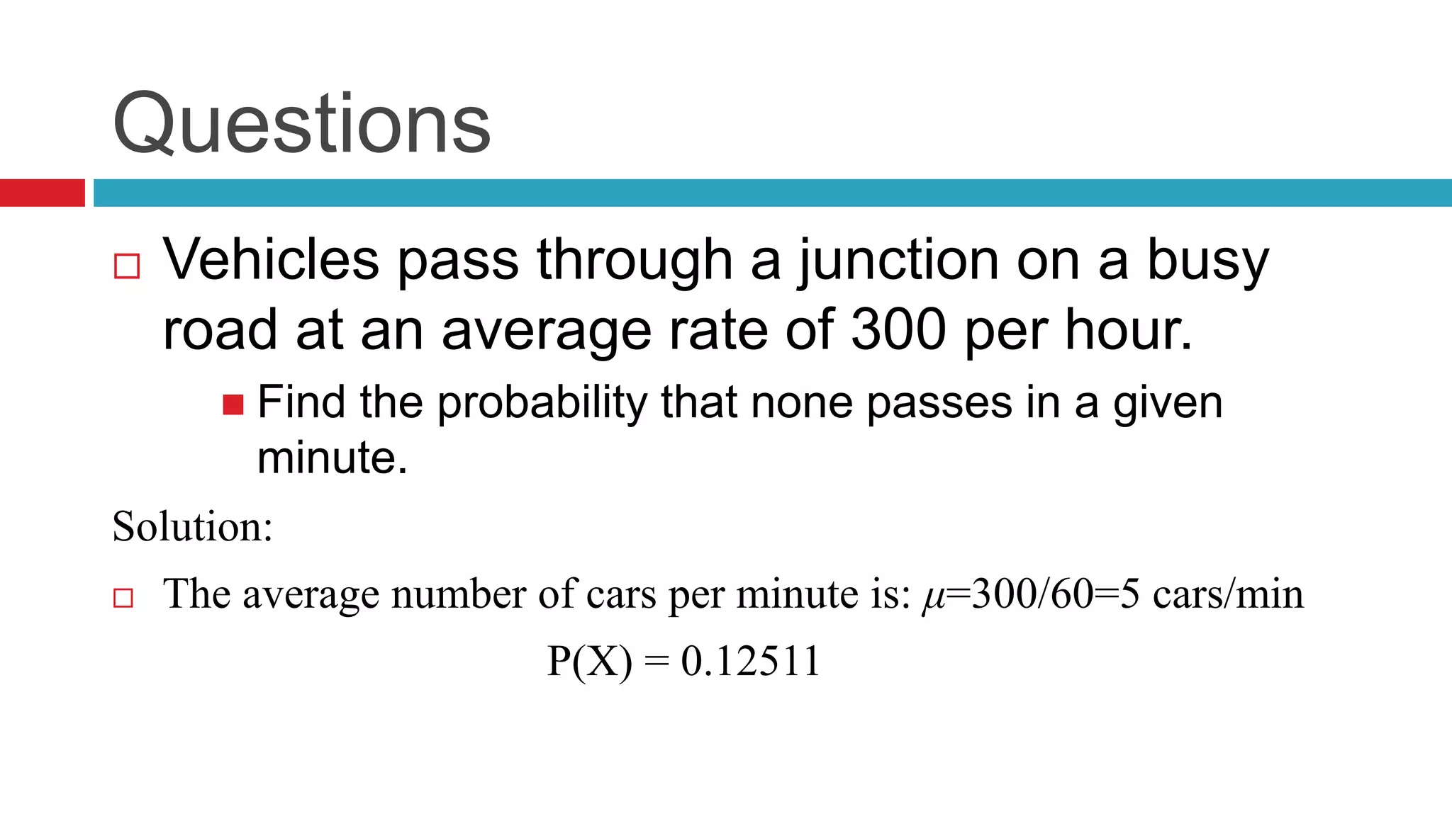
Calculates probability of vehicles passing in a minute based on hourly rates using the Poisson model.
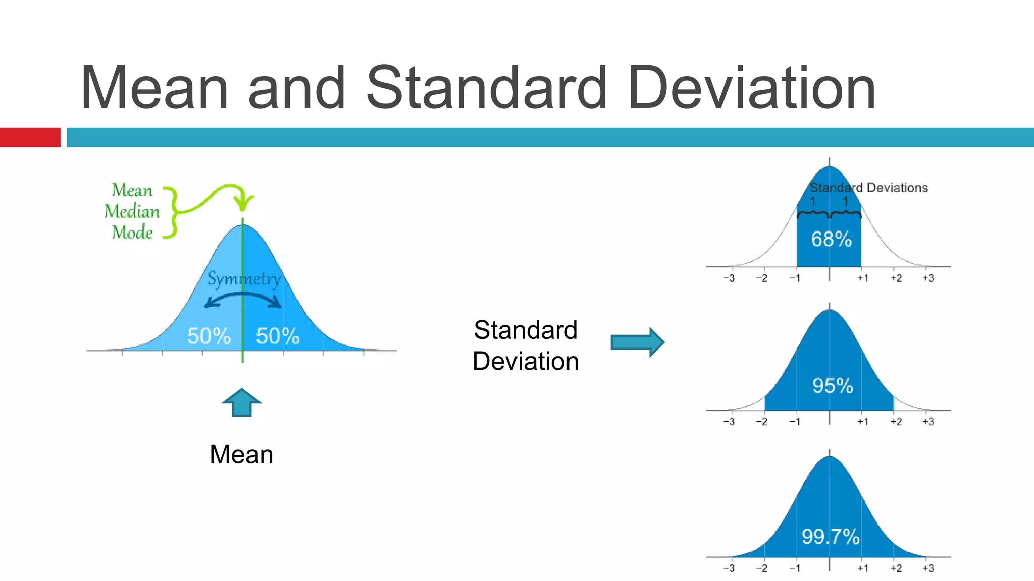
Outlines characteristics of normal distribution, emphasizing symmetrical data distribution and bell-shaped curve.
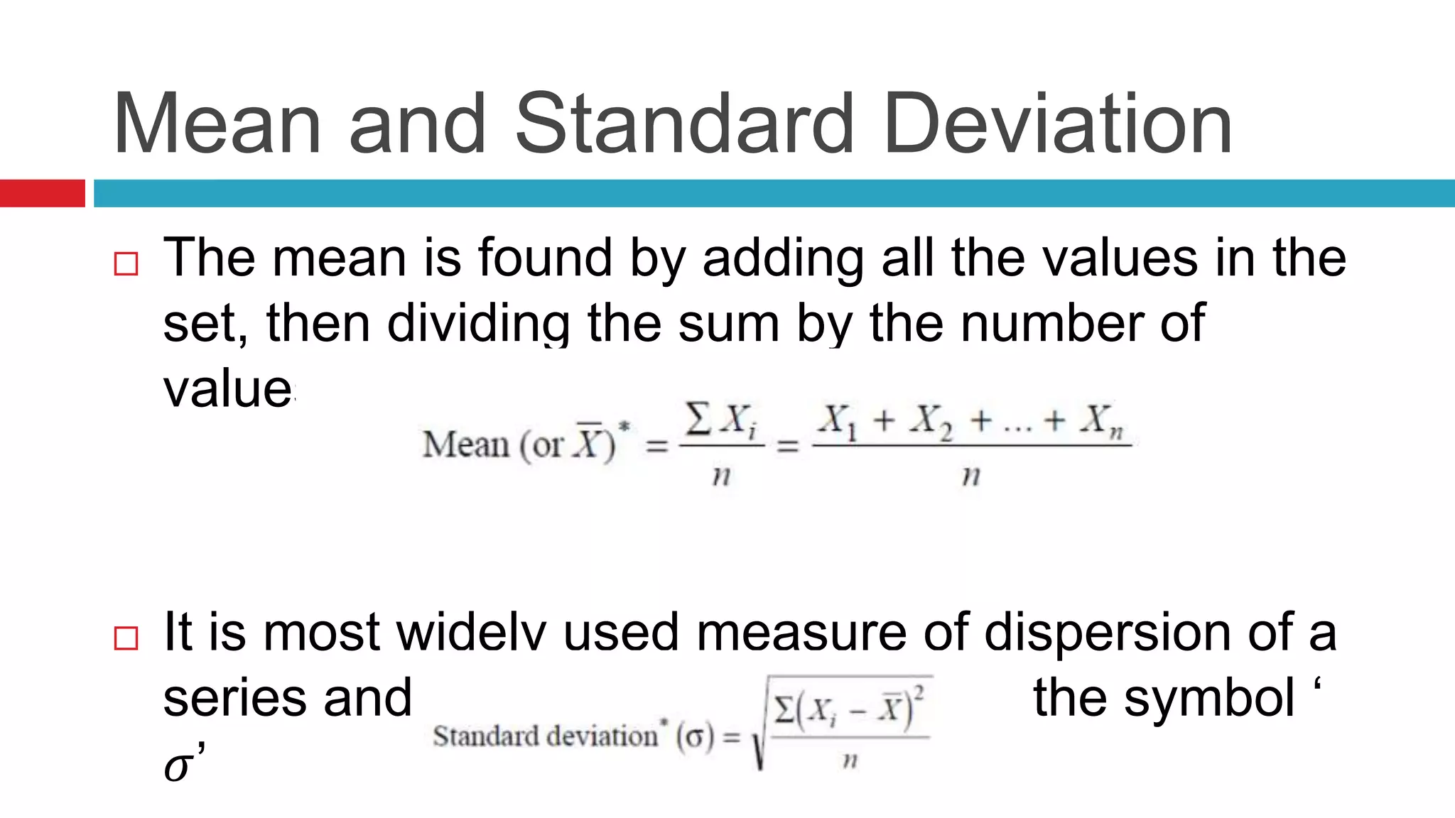
Defines mean and standard deviation; describes their significance in data dispersion and calculation.
Random Variable
Way to map outcomes of random process to numbers.
Random process is a phenomenon that varies to some degree
unpredictably as time goes on. If we observed an entire time-sequence
of the process on several different occasions, under
presumably “identical” conditions, the resulting observation
sequences, in general, would be different.
Examples are flipping a coin, rolling a die.
푋 =
1 푖푓 ℎ푒푎푑 푓푎푙푙
0 푖푓 푡푎푖푙 푓푎푙푙
Mapped the outcome of random process (flipping
coin) and quantified to some variable. (Random
variable)
3.
Types of RandomVariable
Discrete Random Variable
Distinct and separate value. (Can list all the possible value.
i.e., countable)
푋 =
1 푖푓 ℎ푒푎푑 푓푎푙푙
0 푖푓 푡푎푖푙 푓푎푙푙
(possible values are 1 and 0)
Continuous Random Variable
Any value in an interval. Interval may be infinite also.
(Uncountable)
Ex: Mass of random animals selected at Zoo. (Possible
outcomes are uncountable)
4.
Discrete Probability Distribution
X = number of “heads” after 3 flips of fair coins
X is Discrete random variable ( outcomes are 0,1,2
and 3)
Fair coins outcomes : TTT, TTH, THT, THH, HTT,
HTH, HHT, HHH.
P(X=0) = 1/8
P(X=1) = 3/8
P(X=2) = 3/8
P(X=3) = 1/8
This is called as Discrete probability distribution.
5.
Continuous Probability
Distribution
In continuous case, the function f(x) is called
the probability density function, and
probabilities are determined by the areas
under the curve f(x).
Ex: X= Exact amount of rain tomorrow. (may be 1
inches, 2,2.001, 3.1 etc.)
Imagine that probability for all values has given.
6.
Continuous Probability
Distribution
If want to know, what is the probability exactly 2
inches of rain? P(X=2) not 2.0001,1.9999
,2.0000001.not possible.
So we can say 푃( 푋 − 2 < 표. 1). It means
P(1.9<X<2.1). It’s nothing but some area in the
graph.
Based on integral rule, so probabilities are
determined by the areas under the curve.
7.
Discrete Probability Distributionvs
Probability Density Function (PDF)
In Discrete, distribution is Discrete Probability
Distribution and in continuous, the distribution
is PDF.
In PDF, we find probability for some interval
only. (Area of the line is zero)
Sum of all the events probability for both
discrete and continuous is one.
8.
Expected value
The mean (or expected value) of X (is random
variable) gives the value that we would expect
to observe on average in a large number of
repetitions of the experiment
X i x X P x X E
( ) * ( )
1
i
n
i
9.
Example
Aninvestment in Project A will result in a
loss of $26,000 with probability 0.30, break
even with probability 0.50, or result in a profit
of $68,000 with probability 0.20. An
investment in Project B will result in a loss of
$71,000 with probability 0.20, break even
with probability 0.65, or result in a profit of
$143,000 with probability 0.15. Which
investment is better?
10.
Solution
RandomVariable (X)- The amount of money received from
the investment in Project B X can assume only x1 , x2 , x3
X= x1 is the event that we have Loss
X= x2 is the event that we are breaking even
X= x3 is the event that we have a Profit
x1=$-71,000
x2=$0
x3=$143,000
P(X= x1)=0.2
P(X= x2)= 0.65
P(X= x3)= 0.15
11.
Solution
Theamount of money received from the investment
in Project B
X can assume only x1 , x2 , x3
X= x1 is the event that we have Loss
X= x2 is the event that we are breaking even
X= x3 is the event that we have a Profit
x1=$-71,000
x2=$0
x3=$143,000
P(X= x1)=0.2
P(X= x2)= 0.65
P(X= x3)= 0.15
Project B is Better. We made decision using Expected value.
12.
Binomial Distribution
Imagine a simple trial with only two possible outcomes
Success (S)
Failure (F)
Examples
Toss of a coin (heads or tails)
Sex of a newborn (male or female)
Survival of an organism in a region (live or die)
13.
Binomial Distribution
Suppose that the probability of success is p
What is the probability of failure?
q = 1 – p
Examples
Toss of a coin (S = head): p = 0.5 , q = 0.5
Roll of a die (S = 1): p = 0.1667 , q = 0.8333
Fertility of a chicken egg (S = fertile): p = 0.8 , q = 0.2
14.
Binomial Distribution
Imagine that a trial is repeated n times
Examples:
A coin is tossed 5 times
A die is rolled 25 times
50 chicken eggs are examined
Assume p remains constant from trial to trial and that the
trials are independent of each other
15.
Binomial Distribution
What is the probability of obtaining x successes in
n trials?
Example:
What is the probability of obtaining 2 heads from a
coin that was tossed 5 times?
P(HHTTT) = (1/2)^5 = 1/32
16.
Binomial Distribution
Thereare other possibilities also
HHTTT, HTHTT ,HTTHT, HTTTH
THHTT ,THTHT ,THTTH
TTHHT ,TTHTH
TTTHH
Then the probability of x successes is
P(x) = q q p q
= px qn – x
17.
Binomial Distribution
Probability of getting two Head is
P(HHTTT) =
ퟏ
ퟐ
ퟏ
ퟐ
1
2
1
2
1
2
1
2
=
2 1
2
3
How to include other possibilities like HTHTT
etc.,
Order is not important. So multiply with
combination. n!
P(x) = px qn – x
x!(n – x)!
Combination gives
the number of
ways to obtain x
successes in n
18.
Binomial Distribution- Overviews
It is the discrete probability distribution of the number of
successes in a sequence of n independent yes/no
experiments.
A success/failure experiment is also called a Bernoulli
experiment or Bernoulli trial; when n = 1.
The binomial distribution is frequently used to model the
number of successes in a sample of size n drawn with
replacement from a population of size N.
If the sampling is carried out without replacement, the
draws are not independent and so the resulting distribution
is a hypergeometric distribution
19.
Example
Supposeyou independently throw a
dart 10 times. Each time you throw a dart, the
probability of hitting the target is 3/4 . What is
the probability of hitting the target less
than 5 times (out of the total times you throw a
dart)?
Expected value forBinomial
Distribution
E(X) = nP
(Final answer from derivation of expected value
for Binomial Distribution)
The Expected times through the dart is
E(X) = 10*3/4
= 7.5
22.
Poisson Distribution
Discovered by Mathematician Simeon Poisson
in France in 1781.
The modelling distribution that takes his name
was originally derived as an approximation to
the binomial distribution.
n is very large (trial) (n tends to infinity)
P is very small (Probability of success)
23.
Poisson Distribtution
It is an eg of a probability model which is usually
defined by the mean no. of occurrences in a time
interval and simply denoted by λ.
Ex:
Number of telephone calls in a week.
Number of people arriving at a
checkout in a day.
Number of industrial accidents per
month in a manufacturing plant.
24.
When to use?
Occurrences are independent.
Occurrences are random.
The probability of an occurrence is constant
over time.
25.
Poisson Distribution
If we substitute 휆 /n for p, and let n tend to
infinity, the binomial distribution becomes the
Poisson distribution:
P(x) =
e -휆휆x
x!
26.
Example
Aproduction line produces 600 parts per hour
with an average of 5 defective parts an hour. If
you test every part that comes off the line in 15
minutes, what is the probability of finding no
defective parts?
Time interval = 15 minutes
Occurrence rate = 5 defects per hour
27.
Solution
λ =(5 defects/hour)*(0.25 hour)
= 1.25
p(x) = (xe-)/(x!)
x = given number of defects
P(x = 0) = (1.25)0e-1.25)/(0!)
= e-1.25 = 0.287
= 28.7%
28.
Questions
Vehiclespass through a junction on a busy
road at an average rate of 300 per hour.
Find the probability that none passes in a given
minute.
Solution:
The average number of cars per minute is: μ= 300/60=5 cars/min
P(X) = 0.12511
29.
Normal Distribution
The distribution of data happens to be
perfectly symmetrical.
It is perfectly bell shaped curve in which case
the value of mean 푋 = median M = mode Z.
30.
Mean and StandardDeviation
The mean is found by adding all the values in the
set, then dividing the sum by the number of
values.
It is most widely used measure of dispersion of a
series and is commonly denoted by the symbol ‘
휎’