The document provides an overview of random variables, categorizing them into discrete and continuous types. It includes examples of each type and discusses probability distributions, probability mass functions (pmf), and cumulative distribution functions (cdf). The document also features problems to illustrate the concepts of probability related to random variables.

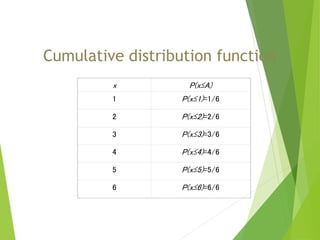
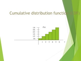
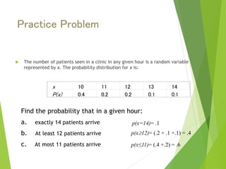
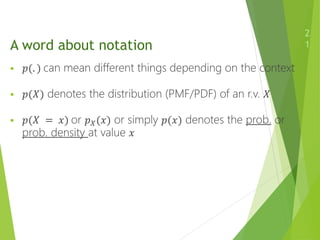
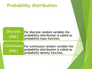
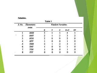
1. Random variables
and its
Characterization
Introduction

2. Random variable
 A numerical value, determined by chance, for
each outcome of a procedure.

3. Random Variable
Let us consider a random experiment of tossing
three coins (or a coin is tossing three times).
Then sample space is
S = {HHH, HHT, HTH, THH, HTT, THT, TTH, TTT}
We are interested in the number of heads in each
outcome.
Let X denote the number of heads in each outcome,
then X takes the values 0,1,2,3

4. Random Variable (Cont.)
X (HHH) = 3, X(HHT) = 2,
X(HTH) = 2, X(THH) = 2 ,
X(HTT) = 1, X (THT) = 1,
X (TTH) = 1, X(TTT) = 0
i.e. X = 0, 1, 2 or 3
X is a variable obtained from the random experiment and is called
random variable.

5. Random variable Types
• A variable that can take
any value which is an
integer values.
• Ex: Position in a class
Discrete
• A variable that can take
any value between the
range.
Ex: Height and weight.
Continuous
5

6. Example: The number of eggs that a hen lays
Another Example
Discrete or Continuous

7. Example: The amount of milk that a cow
produces; e.g. 2.343115 gallons per day
Another Example
Discrete or Continuous

8. Random Variables
 Informally, a random variable (r.v.) 𝑋 denotes possible outcomes of
an event
 Can be discrete (i.e., finite many possible outcomes) or continuous
 Some examples of discrete r.v.
 𝑋 ∈ {0, 1} denoting outcomes of a coin-toss
 𝑋 ∈ {1, 2, . . . , 6} denoting outcome of a dice roll
 Some examples of continuous r.v.
 𝑋 ∈ ℝ denoting heights of students in MTH305
 𝑋 ∈ ℝ denoting time to get to your classroom from Unimall
8
𝑝(𝑋)
𝑝(𝑋)
𝑋(a discrete r.v.)
𝑋(a continuous r.v.)

9. Probability of a random variable
•A probability is usually expressed in terms of a random
variable.
• For the length of a manufactured part, if X denotes the
length. Then the probability statement can be written
in either of the following forms
• Both equations state the probability that the random
variable X assumes a value in [10.8, 11.2] is 0.25.

10. Probability distribution
A description that gives the probability for each value of
the random variable; often expressed in the format of a
graph, table, or formula.

11. Probability Distribution (Example revisited)
Lets find the probability of each outcome in the
example of getting is
P(X = 0) = Probability of getting no head = P(TTT) = 1
8
P(X = 1) = Probability of getting one head
= P(HTT or THT or TTH ) =
3
8
P(X = 2) = Probability of getting two heads
= P(HHT or THH or HTH ) = 3
8
P(X = 3) = Probability of getting three heads
= P(HHH) = 1
8

12. Cont.
Probability distribution of X is:
X 0 1 2 3
1 3 3 1
P(X)
8 8 8 8
P(X) is called the probability distribution
of the random variable X.

13. Discrete Random Variables
 For a discrete r.v. 𝑋, 𝑝(𝑥) denotes
 𝑝(𝑋 = 𝑥) = probability that 𝑋 = 𝑥
 𝑝(𝑋) is called the probability distribution or probabilty mass
function (PMF) of r.v. 𝑋
 𝑝(𝑥) or 𝑝(𝑋 = 𝑥) is the value of the PMF at 𝑥
1
3
𝑝 𝑥 ≥ 0
𝑝 𝑥 ≤ 1
𝑥
𝑝 𝑥 = 1
𝑝(𝑋)
𝑋

14. Cumulative Distribution Function
 Let X be a random variable then
Where P(X ≤ x )is the probability that X is less than or equal to x is
called the cumulative distribution function (d,f.) of X.

15. Properties of Cumulative
Distribution Function.

16. Probability mass function (pmf)
x p(x)
1 p(x=1)=1/6
2 p(x=2)=1/6
3 p(x=3)=1/6
4 p(x=4)=1/6
5 p(x=5)=1/6
6 p(x=6)=1/6
On rolling a dice, following are the probabilities:

17. Discrete example: roll of a die
x
p(x)
1/6
1 4 5 6
2 3
 
x
all
1
P(x)

18. Cumulative distribution function
x P(x≤A)
1 P(x≤1)=1/6
2 P(x≤2)=2/6
3 P(x≤3)=3/6
4 P(x≤4)=4/6
5 P(x≤5)=5/6
6 P(x≤6)=6/6

19. Cumulative distribution function (CDF)
x
P(x)
1/6
1 4 5 6
2 3
1/3
1/2
2/3
5/6
1.0

20. Practice Problem
 The number of patients seen in a clinic in any given hour is a random variable
represented by x. The probability distribution for x is:
x 10 11 12 13 14
P(x) 0.4 0.2 0.2 0.1 0.1
Find the probability that in a given hour:
a. exactly 14 patients arrive
b. At least 12 patients arrive
c. At most 11 patients arrive
p(x=14)= .1
p(x12)= (.2 + .1 +.1) = .4
p(x≤11)= (.4 +.2) = .6

21. A word about notation
2
1
 𝑝(. ) can mean different things depending on the context
 𝑝(𝑋) denotes the distribution (PMF/PDF) of an r.v. 𝑋
 𝑝(𝑋 = 𝑥) or 𝑝𝑋(𝑥) or simply 𝑝(𝑥) denotes the prob. or
prob. density at value 𝑥

22. Probability distribution
For discrete random variable the
probability distribution is called as
probability mass function.
Discrete
(PMF)
For continuous random variable the
probability distribution is called as
probability density function.
Continuous
(PDF)
22

23. Continuous Random Variables
 For a continuous r.v. 𝑋, a probability 𝑝(𝑋 = 𝑥) or 𝑝(𝑥)
is meaningless
 For continuous r.v., prob. Is discussed for an interval
𝑋 ∈ (𝑥, 𝑥 + 𝛿𝑥)
 𝑝(𝑥)𝛿𝑥 is the prob. that 𝑋 ∈ (𝑥, 𝑥 + 𝛿𝑥) as 𝛿𝑥 → 0
 𝑝(𝑥) is the probability density at 𝑋 = 𝑥
𝑝 𝑥 ≥ 0
𝑝 𝑥 𝑑𝑥 = 1

24. For example, the probability of x falling within 1 to 2:
23
.
368
.
135
.
2)
x
P(1 1
2
2
1
2
1












 



 e
e
e
e x
x
x
p(x)=e-x
1
1 2

25. Continuous random variables
 Probability density function

26. Continuous random variables
 Cumulative distribution function

28. s

31. Example
x f(x) p(x)
1 0.2 0.2
2 0.32 0.12
3 0.67 0.35
4 0.9 0.23
5 1 0.1
Total= 1
Hence, P(x=3)=0.35
P(x>2)=1-p(x<=2)
=1-(0.32)
=0.68

32. Example
 Suppose X is a discrete random variable. Let the pmf
of X be given by f(x)=(5-x)/10 for x=1,2,3,4
 Find cdf of X

33. Ex From a lot of 10 items containing 3 defectives, a sample of 4 items
is drawn at random. If X denotes the number of defective items in a
sample.
Solution: Let us consider 10 items as
1 2 3 4 5 6 7 8 9 10
Total number of outcomes if 4 items are selected, is
𝟒
𝟏𝟎
𝑪 = 𝟐𝟏𝟎

34. 1 2 3 4 5 6 7 8 9 10
Let round marked items are defectives
If X denotes the number of defectives, then X=0, 1, 2, 3; since total number of defective
items are 3.
Case 1: No defective
Thus, the number outcomes having no defectives is= 𝟒
𝟕
𝑪. And P(no defective)= 𝟒
𝟕
𝑪
𝟒
𝟏𝟎𝑪
=
𝟏
𝟔
Case 2: 1 defective
(i) {1, 𝟑
𝟕
𝑪}
(ii) {2, 𝟑
𝟕
𝑪}=𝟏
𝟑
𝑪 × 𝟑
𝟕
𝑪
(iii) {3, 𝟑
𝟕
𝑪}
Thus, P(1 defective)=
𝟑×𝟑
𝟕
𝑪
𝟒
𝟏𝟎𝑪
=
𝟏
𝟐

35. Case 3: 2 defectives
(i) {1, 2,𝟐
𝟕
𝑪}
(ii) {1, 3,𝟐
𝟕
𝑪}= 𝟐
𝟑
𝑪 × 𝟐
𝟕
𝑪 = 𝟑 × 𝟐
𝟕
𝑪
(iii) {2, 3, 𝟑
𝟕
𝑪}
Thus, P(2 defectives)=
𝟑×𝟐
𝟕
𝑪
𝟒
𝟏𝟎𝑪
=
𝟑
𝟏𝟎
Case 4: 3 defectives
There are 7 such cases {1,2,3,4}; {1,2,3,5}; {1,2,3,6}, {1,2,3,7}, {1,2,3,8}, {1,2,3,9}, {1,2,3,10}
Thus, P(3 defectives)= 𝟏
𝟕
𝑪 𝟑
𝟑
𝑪
𝟒
𝟏𝟎𝑪
=
𝟕
𝟒
𝟏𝟎𝑪
=
𝟏
𝟑𝟎
Thus probability distribution is
X 0 1 2 3
P(x)=f(x) 1/6 1/2 3/10 1/30

36. (ii) Now, 𝑃 𝑥 ≤ 1 = 𝑃 0 + 𝑃 1 =
2
3
; 𝑃 𝑥 < 1 = 𝑃 0 =
1
6
; 𝑃 0 < 𝑥 < 2 = 𝑃 1 = 1/2

37. Important Examples

40. Try by yourself
 Probability function of (ii)Y (iii) Z, (iv) X +Y and (v) XY

41. z

42. To draw Probability chart

43. Example
 The probability density function of a random
variable x is given as:
𝑓(𝑥) = 𝑘(𝑥 − 1)(2 − 𝑥) for 1 ≤ 𝑥 ≤ 2 .
Determine
i) the value of the constant k.
ii) the distribution function F(x)
iii) 𝑃(5/4≤ 𝑥 ≤ 3/2)

45. 1

48. Example
A random variable is exponentially distributed with
probability distribution function as
𝑓 𝑥 =
1
40
𝑒−
𝑥
40 𝑓𝑜𝑟 𝑥 > 0
=0 𝑓𝑜𝑟 𝑥 ≤ 0
Find
i) P X ≤ 20
ii) P 32 ≤ X ≤ 48
iii)P X ≥ 25

50. Thank You...