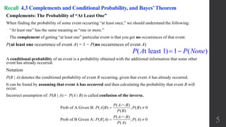
Download to read offline


![Parameters of a Probability Distribution
Remember that with a probability distribution, we have a description of a population
instead of a sample, so the values of the mean, standard deviation, and variance are
parameters, not statistics.
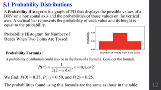
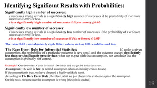
The mean, variance, and standard deviation of a discrete probability distribution can be
found with the following formulas:
Mean (Expected Value), Variance & Standard Deviation of D.R.V x:
Mean (the expected value) of occurrence per repetition (it represents the average
value of the outcome):
14
5.1 Probability Distributions μ = 𝐸 𝑥 = 𝑥𝑝(𝑥)
2 2 2
2 2 2
2
2 2 2
( ) ( )
( ) ( ) ( ) ,
( ) ( ) ( 2 ) ( )
( ) [2 ( ) ( )]
( ) [2 1] ( )
Pr
E x xp x
x p x x p x
x p x x x p x
x p x xp x p x
x x p
f
p x x
oo
Mean: ( )x P x
2 2 2
Variance: ( )x P x ](https://image.slidesharecdn.com/5-190813004531/85/Probability-distributions-14-320.jpg)


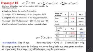

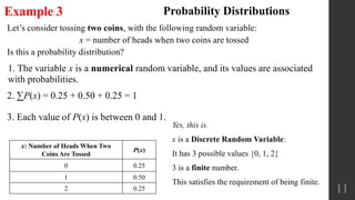
Okay, let's solve this step-by-step: 1) Define the random variable: X = Number of trips of 5 days or more per year 2) Write the probability distribution: x P(x) 0 0.06 1 0.70 2 0.20 3 0.03 3) Calculate the mean using the formula: Mean = Σx * P(x) 0 * 0.06 + 1 * 0.70 + 2 * 0.20 + 3 * 0.03 = 0.84 So the mean number of trips per year is 0.84.