Chapter 7 Random Variables & Probability Distributions
Random Variables A numerical variable whose value depends on the outcome of a chance experiment is called a  random variable . A random variable associates a numerical value with each outcome of a chance experiment.
A random variable is  discrete  if its set of possible values is a collection of isolated points on the number line. Discrete and Continuous Random Variables A random variable is  continuous  if its set of possible values includes an entire interval on the number line. We will use lowercase letters, such as x and y, to represent random variables. Possible values of a discrete random variable Possible values of a continuous random variable
Examples 1. Experiment: A fair die is rolled Random Variable: The number on the up face Type: Discrete 2. Experiment: A pair of fair dice are rolled Random Variable: The sum of the up faces Type: Discrete Another random variable: The smaller of the up faces Type: Discrete
Examples 3. Experiment: A coin is tossed until the 1 st  head turns up Random Variable: The number of the toss that the 1 st  head turns up Type: Discrete 4. Experiment: Choose and inspect a number of parts  Random Variable: The number of defective parts Type: Discrete
5. Experiment: Inspect a precision ground mirror (Hubbell?) Random Variable: The number of defects on the surface of the mirror Type: Discrete 6. Experiment: Measure the resistance of a '5' ohm resistor Random Variable: The resistance (in ohms) Type: Continuous Examples
7. Experiment: Measure the voltage in a outlet in your room Random Variable: The voltage Type: Continuous 8. Experiment: Observe the amount of time it takes a bank teller to serve a customer Random Variable: The time Type: Continuous Examples
9. Experiment: Measure the time until the next customer arrives at a customer service window Random Variable: The time Type: Continuous 10. Experiment: Inspect a randomly chosen circuit board from a production line Random Variable: 1, if the circuit board is defective 0, if the circuit board is not defective Type: Discrete Examples
Discrete Probability Distributions The  probability distribution of a discrete random variable x  gives the probability associated with each possible x value.  Each probability is the limiting relative frequency of occurrence of the corresponding x value when the experiment is repeatedly performed.
Example Suppose that 20% of the apples sent to a sorting line are Grade A.  If 3 of the apples sent to this plant are chosen randomly, determine the probability distribution of the number of Grade A apples in a sample of 3 apples.  Consider the tree diagram A A C .8 .2 A A C .8 .2 A A C .8 .2 A A C .8 .2 A A C .8 .2 A A C .8 .2 A A C .8 .2 .2  .2  .2=.008 .2  .2  .8=.032 .2  .8  .2=.032 .2  .8  .8=.128 .8  .2  .2=.032 .8  .2  .8=.128 .8  .8  .2=.128 .8  .8  .8=.512 3 X 2 2 1 2 1 1 0
The Results in Table Form or
Results in Graphical Form (Probability Histogram) For a probability histogram, the area of a bar is the probability of obtaining that value associated with that bar.
The probabilities p i  must satisfy 1.   0  ≤  p i   ≤  1 for each i 2.   p 1  + p 2  + ... + p k  = 1 The probability P(X in A) of any event is found by summing the p i  for the outcomes x i  making up A. Probability Distributions
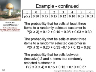
Example The number of items a given salesman sells per customer is a random variable.  The table below is for a specific salesman (Wilbur) in a clothing store in the mall.  The probability distribution of X is given below: Note: 0  ≤  p(x)  ≤  1 for each x  p(x) = 1 (the sum is over all values of x) x 0 1 2 3 4 5 6 p(x) 0.20 0.35 0.15 0.12 0.10 0.05 0.03
Example - continued The probability that he sells at least three items to a randomly selected customer is P(X  ≥  3) = 0.12 + 0.10 + 0.05 + 0.03 = 0.30 The probability that he sells at most three items to a randomly selected customer is P(X  ≤  3) = 0.20 + 0.35 +0.15 + 0.12 = 0.82 The probability that he sells between (inclusive) 2 and 4 items to a randomly selected customer is P(2  ≤  X  ≤  4) = 0.15 + 0.12 + 0.10 = 0.37 x 0 1 2 3 4 5 6 p(x) 0.20 0.35 0.15 0.12 0.10 0.05 0.03
Probability Histogram A probability histogram has its vertical scale adjusted in a manner that makes the area associated with each bar equal to the probability of the event that the random variable takes on the value describing the bar.
Continuous Probability Distributions If one looks at the distribution of the actual amount of water (in ounces) in “one gallon” bottles of spring water they might see something such as Amount measured to nearest ten thousands of an ounce.  Amount measured to nearest hundredths of an ounce.  Limiting curve as the accuracy increases
Probability Distribution for a Continuous Random Variable A  probability distribution for a continuous random variable x  is specified by a mathematical function denoted by f(x) which is called the  density function . The graph of a density function is a smooth curve (the  density curve ).  The following requirements must be met: f(x)    0  The total area under the density curve is equal to 1. The probability that x falls in any particular interval is the area under the density curve that lies above the interval.
Some Illustrations Notice that for a continuous random variable x,  P(x = a) = 0 for any specific value a because the “area above a point” under the curve is a line segment and hence has o area.  Specifically this means P(x < a) = P(x  ≤  a). a P(x < a) a P(x < a)
Some Illustrations Note: P(a < x < b) = P(a  ≤ x < b)  = P(a < x ≤ b)  = P(a ≤ x ≤ b) b a a b a b P(a < x < b) P(a < x < b) P(a < x < b)
Some Illustrations P(x > b) = P(b < x) b b P(x > b) = P(b < x)
Example Define a continuous random variable x by  x = the weight of the crumbs in ounces left on the floor of a restaurant during a one hour period.  Suppose that x has a probability distribution with density function 1 2 3 4 5 6 7 .25 The graph looks like
Example Find the probability that during a given 1 hour period between 3 and 4.5 ounces of crumbs are left on the restaurant floor. The probability is represented by the shaded area in the graph. Since that shaded area is a rectangle, area = (base)(height)=(1.5)(.25) = .375 1 2 3 4 5 6 7 .25
Method of Probability Calculation The probability that a continuous random variable x lies between a lower limit a and an upper limit b is P(a < x < b) = (cumulative area to the left of b) –  (cumulative area to the left of a) = P(x < b) – P(x < a) = - a b a b
Mean & Standard Deviation The  mean value of a random variable x , denoted by   x , describes where the probability distribution of x is centered. The  standard deviation of a random variable x , denoted by   x , describes variability in the probability distribution.  When   x  is small, observed values of x will tend to be close to the mean value and  when   x  is large, there will be more variability in observed values.
Illustrations Two distributions with the same standard deviation with different means. Larger mean
Illustrations Two distributions with the same means and different standard deviation. Smaller standard deviation
Mean of a Discrete Random Variable The  mean value of a discrete random variable x , denoted by   x , is computed by first multiplying each possible x value by the probability of observing that value and then adding the resulting quantities. Symbolically,
Example A professor regularly gives multiple choice quizzes with 5 questions. Over time, he has found the distribution of the number of wrong answers on his quizzes is as follows
Example Multiply each x value by its probability and add the results to get   x .  x  = 1.41
Variance and Standard Deviation of a Discrete Random Variable
Previous Example - continued
The Mean & Variance of a Linear Function
Example Suppose x is the number of sales staff needed on a given day.  If the cost of doing business on a day involves fixed costs of $255 and the cost per sales person per day is $110, find the mean cost (the mean of x or   x ) of doing business on a given day where the distribution of x is given below.
Example continued We need to find the mean of  y = 255 + 110x
Example continued We need to find the variance and standard deviation of  y = 255 + 110x
Means and Variances for Linear Combinations If x 1 , x 2 ,    , x n  are random variables and a 1 , a 2 ,    , a n  are numerical constants, the random variable y defined as y = a 1 x 1  + a 2 x 2  +    + a n x n is a  linear combination of the x i ’s.
Means and Variances for Linear Combinations 1.  y  = a 1  1  + a 2  2  +    + a n  n   (This is true for any random variables with no conditions.) If x 1 , x 2 ,    , x n  are random variables with means   1 ,   2 ,    ,   n  and variances  respectively,  and  y = a 1 x 1  + a 2 x 2  +    + a n x n   then 2. If x 1 , x 2 ,    , x n  are  independent  random variables then and
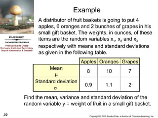
Example A distributor of fruit baskets is going to put 4 apples, 6 oranges and 2 bunches of grapes in his small gift basket. The weights, in ounces, of these items are the random variables x 1 , x 2  and x 3  respectively with means and standard deviations as given in the following table. Find the mean, variance and standard deviation of the random variable y = weight of fruit in a small gift basket. Apples Oranges Grapes Mean  8 10 7 Standard deviation  0.9 1.1 2
Example continued It is reasonable in this case to assume that the weights of the different types of fruit are  independent . Apples Oranges Mean  8 10 7 Standard deviation  0.9 1.1 2 Grapes
Another Example Suppose “1 lb” boxes of Sugar Treats cereal have a weight distribution with a mean   T =1.050 lbs and standard deviation   T =.051 lbs and “1 lb” boxes of Sour Balls cereal have a weight distribution with a mean   B =1.090 lbs and standard deviation   B =.087 lbs. If a promotion is held where the customer is sold a shrink wrapped package containing “1 lb” boxes of both Sugar Treats and Sour Balls cereals, what is the mean and standard deviation for the distribution of promotional packages.
Another Example - continued Combining these values we get Combining these values we get
The Binomial Distribution Properties of a Binomial Experiment It consists of a fixed number of observations called trials. Each trial can result in one of only two mutually exclusive outcomes labeled success (S) and failure (F). Outcomes of different trials are independent. The probability that a trial results in S is the same for each trial. The  binomial random variable  x is defined as x = number of successes observed when    experiment is performed The probability distribution of x is called the  binomial probability distribution .
The Binomial Distribution Let  n = number of independent trials in a binomial experiment    = constant probability that any particular trial results in a success. Then
Example The adult population of a large urban area is 60% black. If a jury of 12 is randomly selected from the adults in this area, what is the probability that precisely 7 jurors are black. Clearly, n=12 and   =.6, so 0.2270 ) 4 (. ) 6 (. ! 5 ! 7 ! 12 ) 7 ( p 5 7  
Example - continued The adult population of a large urban area is 60% black. If a jury of 12 is randomly selected from the adults in this area, what is the probability that less than 3 are black. Clearly, n = 12 and   = 0.6, so
Another Example a) What is the probability that exactly two will respond favorably to this sales pitch? On the average, 1 out of 19 people will respond favorably to a certain telephone solicitation.  If 25 people are called,
Another Example continued On the average, 1 out of 19 people will respond favorably to a certain telephone sales pitch.  If 25 people are called,  b) What is the probability that at least two will respond favorably to this sales pitch?
Mean & Standard Deviation of a Binomial Random Variable The mean value and the standard deviation of a binomial random variable are, respectively,
Example A professor routinely gives quizzes containing 50 multiple choice questions with 4 possible answers, only one being correct.  Occasionally he just hands the students an answer sheet without giving them the questions and asks them to guess the correct answers.  Let x be a random variable defined by x = number of correct answers on such an exam Find the mean and standard deviation for x
Example - solution The random variable is clearly binomial with n = 50 and p = ¼. The mean and standard deviation of x are
The Geometric Distribution Suppose an experiment consists of a sequence of trials with the following conditions: The trials are independent. Each trial can result in one of two possible outcomes, success and failure. The probability of success is the same for all trials. A  geometric random variable  is defined as x = number of trials until the first success is observed (including the success trial) The probability distribution of x is called the  geometric probability distribution.
The Geometric Distribution If x is a geometric random variable with probability of success =    for each trial, then  p(x) = (1 –   ) x-1    x = 1, 2, 3,  …
Example Over a very long period of time, it has been noted that on Friday’s 25% of the customers at the drive-in window at the bank make deposits. What is the probability that it takes 4 customers at the drive-in window before the first one makes a deposit.
Example - solution This problem is a geometric distribution problem with    = 0.25. Let x = number of customers at the drive-in window before a customer makes a deposit. The desired probability is
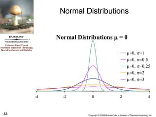
Normal Distributions Two characteric values (numbers) completely determine a normal distribution Mean  -  µ Standard deviation  -  
Normal Distributions
Major Principle The proportion or percentage of a normally distributed population that is in an interval depends only on how many standard deviations the endpoints are from the mean.
Standard Normal Distribution A normal distribution with mean 0 and standard deviation 1, is called the standard (or standardized) normal distribution.
Normal Tables
Normal Tables
Using the Normal Tables For any number z* between –3.89 and 3.89 and rounded to two decimal places, Appendix Table II gives  (Area under z curve to the left of z*)  = P(z < z*) = P(z     z*) where the letter z is used to represent a random variable whose distribution is the standard normal distribution
Using the Normal Tables To find this probability, locate the following: The row labeled with the sign of z* and the digit to either side of the decimal point  The column identified with the second digit to the right of the decimal point in z* The number at the intersection of this row and column is the desired probability, P(z < z*).
Using the Normal Tables Find P(z < 0.46) Row labeled 0.4 Column labeled 0.06 P(z < 0.46) = 0.6772
Using the Normal Tables Find P(z < -2.74) Row labeled -2.7 Column labeled 0.04 P(z < -2.74) = 0.0031
Sample Calculations Using the Standard Normal Distribution Using the standard normal tables, find the proportion of observations (z values) from a standard normal distribution that satisfy each of the following: P(z < 1.83) = 0.9664 (b) P(z > 1.83) = 1 – P(z < 1.83) = 1 – 0.9664 = 0.0336
Sample Calculations Using the Standard Normal Distribution Using the standard normal tables, find the proportion of observations (z values) from a standard normal distribution that satisfies each of the following: c) P(z < -1.83) = 0.0336  (d) P(z > -1.83) = 1 – P(z < -1.83) = 1 – 0.0336= 0.9664
Symmetry Property Notice from the preceding examples it becomes obvious that  P(z > z*) = P(z < -z*) P(z > -2.18) = P(z < 2.18) = 0.9854
Sample Calculations Using the Standard Normal Distribution Using the standard normal tables, find the proportion of observations (z values) from a standard normal distribution that satisfies  -1.37 < z < 2.34, that is find P(-1.37 < z < 2.34). P(Z<2.34)=0.9904 P(-1.37 < z < 2.34) = 0.9904 P(Z<-1.37)=0.0853 - 0.0853 = 0.9051
Sample Calculations Using the Standard Normal Distribution Using the standard normal tables, find the proportion of observations (z values) from a standard normal distribution that satisfies  0.54 < z < 1.61, that is find P(0.54 < z < 1.61). P(0.54 < z < 1.61) = 0.9463 P(Z<1.61)=0.9463 P(Z<.54)=0.7054 - 0.7054 = 0.2409
Sample Calculations Using the Standard Normal Distribution Using the standard normal tables, find the proportion of observations (z values) from a standard normal distribution that satisfy -1.42 < z < -0.93, that is find P(-1.42 < z < -0.93). P(Z<-0.93)=0.1762 P(-1.42 < z < -0.93) = 0.1762 P(Z<-1.42)=0.0778 - 0.0778 = 0.0984
Example Calculation Using the standard normal tables, in each of the following, find the z values that satisfy : The closest entry in the table to 0.9800 is 0.9798 corresponding to a z value of 2.05 (a) The point z with 98% of the observations  falling below it.
Example Calculation Using the standard normal tables, in each of the following, find the z values that satisfy : (b) The point z with 90% of the observations  falling above it. The closest entry in the table to 0.1000 is 0.1003 corresponding to a z value of -1.28
Finding Normal Probabilities To calculate probabilities for any normal distribution, standardize the relevant values and then use the table of z curve areas. More specifically, if x is a variable whose behavior is described by a normal distribution with mean m and standard deviation s, then P(x < b) = p(z < b*) P(x > a) = P(a* < z) = P(z > a*)  where z is a variable whose distribution is standard normal and
Standard Normal Distribution Revisited This is called the  standard normal distribution. If a variable X has a normal distribution with mean    and standard deviation   , then the standardized variable has the normal distribution with mean 0 and standard deviation 1.
Conversion to N(0,1) Where    is the true population mean and    is the true population standard deviation The formula gives the number of standard deviations that x is from the mean.
Example 1 A Company produces “20 ounce” jars of a picante sauce.  The true amounts of sauce in the jars of this brand sauce follow a normal distribution. Suppose the companies “20 ounce” jars follow a N(20.2,0.125) distribution curve. (i.e., The contents of the jars are normally distributed with a true mean   = 20.2 ounces with a true standard deviation   = 0.125 ounces.
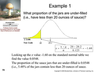
Example 1 What proportion of the jars are under-filled  (i.e., have less than 20 ounces of sauce)? Looking up the z value -1.60 on the standard normal table we find the value 0.0548. The proportion of the sauce jars that are under-filled is 0.0548 (i.e., 5.48% of the jars contain less than 20 ounces of sauce.
Example 1 What proportion of the sauce jars contain between 20 and 20.3 ounces of sauce. Looking up the z values of -1.60 and 0.80 we find the areas (proportions) 0.0548 and 0.7881 The resulting difference  0.7881-0.0548 = 0.7333  is the proportion of the jars that contain between 20 and 20.3 ounces of sauce.
Example 1 99% of the jars of this brand of picante sauce will contain more than what amount of sauce? When we try to look up 0.0100 in the body of the table we do not find this value.  We do find the following Since the relationship between the real scale (x) and the z scale is z=(x-  )/   we solve for x getting x =   + z  x=20.2+(-2.33)(0.125)= 19.90875=19.91 The entry closest to 0.0100 is 0.0099 corresponding to the z value -2.33
The weight of the cereal in a box is a random variable with mean 12.15 ounces, and standard deviation 0.2 ounce.  What percentage of the boxes have contents that weigh under 12 ounces?  Example 2
If the manufacturer claims there are 12 ounces in a box, does this percentage cause concern?  If so, what could be done to correct the situation?  The machinery could be reset with a higher or larger  mean. The machinery could be replaced with machinery that has a smaller standard deviation of fills. The label on the box could be changed. Which would probably be cheaper immediately but might cost more in the long run? In the long run it might be cheaper to get newer more precise equipment and not give away as much excess cereal. Example 2
Example 3 a) What proportion of these printers will fail before 1,200 hours? The time to first failure of a unit of a brand of ink jet printer is approximately normally distributed with a mean of 1,500 hours and a standard deviation of 225 hours.
Example 3 b) What proportion of these printers will not fail within the first 2,000 hours?
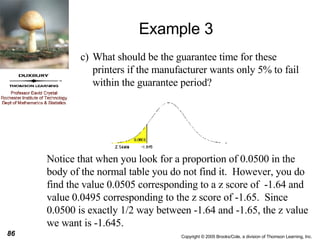
Example 3 c) What should be the guarantee time for these printers if the manufacturer wants only 5% to fail within the guarantee period? Notice that when you look for a proportion of 0.0500 in the body of the normal table you do not find it.  However, you do find the value 0.0505 corresponding to a z score of  -1.64 and value 0.0495 corresponding to the z score of -1.65.  Since 0.0500 is exactly 1/2 way between -1.64 and -1.65, the z value we want is -1.645.
Example 3 The guarantee period should be 1130 hours. The relationship connecting x, z,   and    is .  If you solve this equation for x you get  x =    + z   , so
Normal Plots A  normal probability plot  is a scatter plot of the (normal score * , observation) pairs. A substantially linear pattern in a normal probability plot suggests that population normality is plausible. A systematic departure from a straight-line pattern (such as curvature in the plot) casts doubt on the legitimacy of assuming a normal population distribution. * There are different techniques for determining the normal scores. Typically, we use a statistical package such as Minitab, SPSS or SAS to create a normal probability plot.
Normal Probability Plot Example Ten randomly selected shut-ins were each asked to list how many hours of television they watched per week.  The results are 82 66 90 84 75 88 80 94 110 91 Minitab obtained the normal probability plot on the following slide.
Normal Probability Plot Example Notice that the points all fall nearly on a line so it is reasonable to assume that the population of hours of tv watched by shut-ins is normally distributed.
Normal Probability Plot Example A sample of times of 15 telephone solicitation calls (in seconds) was obtained and is given below. 5 10 7 12 35 65 145 14 3 220 11 6 85 6 16   Minitab obtained the normal probability plot on the next slide
Normal Probability Plot Example Clearly the points do not fall nearly on a line. Specifically the pattern has a distinct nonlinear appearance. It is  not  reasonable to assume that the population of hours of tv watched by shut-ins is normally distributed.  One would most assuredly say that the distribution of lengths of calls is not normal.
Chapter07

  • 1.
    Chapter 7 RandomVariables & Probability Distributions
  • 2.
    Random Variables Anumerical variable whose value depends on the outcome of a chance experiment is called a random variable . A random variable associates a numerical value with each outcome of a chance experiment.
  • 3.
    A random variableis discrete if its set of possible values is a collection of isolated points on the number line. Discrete and Continuous Random Variables A random variable is continuous if its set of possible values includes an entire interval on the number line. We will use lowercase letters, such as x and y, to represent random variables. Possible values of a discrete random variable Possible values of a continuous random variable
  • 4.
    Examples 1. Experiment:A fair die is rolled Random Variable: The number on the up face Type: Discrete 2. Experiment: A pair of fair dice are rolled Random Variable: The sum of the up faces Type: Discrete Another random variable: The smaller of the up faces Type: Discrete
  • 5.
    Examples 3. Experiment:A coin is tossed until the 1 st head turns up Random Variable: The number of the toss that the 1 st head turns up Type: Discrete 4. Experiment: Choose and inspect a number of parts Random Variable: The number of defective parts Type: Discrete
  • 6.
    5. Experiment: Inspecta precision ground mirror (Hubbell?) Random Variable: The number of defects on the surface of the mirror Type: Discrete 6. Experiment: Measure the resistance of a '5' ohm resistor Random Variable: The resistance (in ohms) Type: Continuous Examples
  • 7.
    7. Experiment: Measurethe voltage in a outlet in your room Random Variable: The voltage Type: Continuous 8. Experiment: Observe the amount of time it takes a bank teller to serve a customer Random Variable: The time Type: Continuous Examples
  • 8.
    9. Experiment: Measurethe time until the next customer arrives at a customer service window Random Variable: The time Type: Continuous 10. Experiment: Inspect a randomly chosen circuit board from a production line Random Variable: 1, if the circuit board is defective 0, if the circuit board is not defective Type: Discrete Examples
  • 9.
    Discrete Probability DistributionsThe probability distribution of a discrete random variable x gives the probability associated with each possible x value. Each probability is the limiting relative frequency of occurrence of the corresponding x value when the experiment is repeatedly performed.
  • 10.
    Example Suppose that20% of the apples sent to a sorting line are Grade A. If 3 of the apples sent to this plant are chosen randomly, determine the probability distribution of the number of Grade A apples in a sample of 3 apples. Consider the tree diagram A A C .8 .2 A A C .8 .2 A A C .8 .2 A A C .8 .2 A A C .8 .2 A A C .8 .2 A A C .8 .2 .2  .2  .2=.008 .2  .2  .8=.032 .2  .8  .2=.032 .2  .8  .8=.128 .8  .2  .2=.032 .8  .2  .8=.128 .8  .8  .2=.128 .8  .8  .8=.512 3 X 2 2 1 2 1 1 0
  • 11.
    The Results inTable Form or
  • 12.
    Results in GraphicalForm (Probability Histogram) For a probability histogram, the area of a bar is the probability of obtaining that value associated with that bar.
  • 13.
    The probabilities pi must satisfy 1. 0 ≤ p i ≤ 1 for each i 2. p 1 + p 2 + ... + p k = 1 The probability P(X in A) of any event is found by summing the p i for the outcomes x i making up A. Probability Distributions
  • 14.
    Example The numberof items a given salesman sells per customer is a random variable. The table below is for a specific salesman (Wilbur) in a clothing store in the mall. The probability distribution of X is given below: Note: 0 ≤ p(x) ≤ 1 for each x  p(x) = 1 (the sum is over all values of x) x 0 1 2 3 4 5 6 p(x) 0.20 0.35 0.15 0.12 0.10 0.05 0.03
  • 15.
    Example - continuedThe probability that he sells at least three items to a randomly selected customer is P(X ≥ 3) = 0.12 + 0.10 + 0.05 + 0.03 = 0.30 The probability that he sells at most three items to a randomly selected customer is P(X ≤ 3) = 0.20 + 0.35 +0.15 + 0.12 = 0.82 The probability that he sells between (inclusive) 2 and 4 items to a randomly selected customer is P(2 ≤ X ≤ 4) = 0.15 + 0.12 + 0.10 = 0.37 x 0 1 2 3 4 5 6 p(x) 0.20 0.35 0.15 0.12 0.10 0.05 0.03
  • 16.
    Probability Histogram Aprobability histogram has its vertical scale adjusted in a manner that makes the area associated with each bar equal to the probability of the event that the random variable takes on the value describing the bar.
  • 17.
    Continuous Probability DistributionsIf one looks at the distribution of the actual amount of water (in ounces) in “one gallon” bottles of spring water they might see something such as Amount measured to nearest ten thousands of an ounce. Amount measured to nearest hundredths of an ounce. Limiting curve as the accuracy increases
  • 18.
    Probability Distribution fora Continuous Random Variable A probability distribution for a continuous random variable x is specified by a mathematical function denoted by f(x) which is called the density function . The graph of a density function is a smooth curve (the density curve ). The following requirements must be met: f(x)  0 The total area under the density curve is equal to 1. The probability that x falls in any particular interval is the area under the density curve that lies above the interval.
  • 19.
    Some Illustrations Noticethat for a continuous random variable x, P(x = a) = 0 for any specific value a because the “area above a point” under the curve is a line segment and hence has o area. Specifically this means P(x < a) = P(x ≤ a). a P(x < a) a P(x < a)
  • 20.
    Some Illustrations Note:P(a < x < b) = P(a ≤ x < b) = P(a < x ≤ b) = P(a ≤ x ≤ b) b a a b a b P(a < x < b) P(a < x < b) P(a < x < b)
  • 21.
    Some Illustrations P(x> b) = P(b < x) b b P(x > b) = P(b < x)
  • 22.
    Example Define acontinuous random variable x by x = the weight of the crumbs in ounces left on the floor of a restaurant during a one hour period. Suppose that x has a probability distribution with density function 1 2 3 4 5 6 7 .25 The graph looks like
  • 23.
    Example Find theprobability that during a given 1 hour period between 3 and 4.5 ounces of crumbs are left on the restaurant floor. The probability is represented by the shaded area in the graph. Since that shaded area is a rectangle, area = (base)(height)=(1.5)(.25) = .375 1 2 3 4 5 6 7 .25
  • 24.
    Method of ProbabilityCalculation The probability that a continuous random variable x lies between a lower limit a and an upper limit b is P(a < x < b) = (cumulative area to the left of b) – (cumulative area to the left of a) = P(x < b) – P(x < a) = - a b a b
  • 25.
    Mean & StandardDeviation The mean value of a random variable x , denoted by  x , describes where the probability distribution of x is centered. The standard deviation of a random variable x , denoted by  x , describes variability in the probability distribution. When  x is small, observed values of x will tend to be close to the mean value and when  x is large, there will be more variability in observed values.
  • 26.
    Illustrations Two distributionswith the same standard deviation with different means. Larger mean
  • 27.
    Illustrations Two distributionswith the same means and different standard deviation. Smaller standard deviation
  • 28.
    Mean of aDiscrete Random Variable The mean value of a discrete random variable x , denoted by  x , is computed by first multiplying each possible x value by the probability of observing that value and then adding the resulting quantities. Symbolically,
  • 29.
    Example A professorregularly gives multiple choice quizzes with 5 questions. Over time, he has found the distribution of the number of wrong answers on his quizzes is as follows
  • 30.
    Example Multiply eachx value by its probability and add the results to get  x .  x = 1.41
  • 31.
    Variance and StandardDeviation of a Discrete Random Variable
  • 32.
  • 33.
    The Mean &Variance of a Linear Function
  • 34.
    Example Suppose xis the number of sales staff needed on a given day. If the cost of doing business on a day involves fixed costs of $255 and the cost per sales person per day is $110, find the mean cost (the mean of x or  x ) of doing business on a given day where the distribution of x is given below.
  • 35.
    Example continued Weneed to find the mean of y = 255 + 110x
  • 36.
    Example continued Weneed to find the variance and standard deviation of y = 255 + 110x
  • 37.
    Means and Variancesfor Linear Combinations If x 1 , x 2 ,  , x n are random variables and a 1 , a 2 ,  , a n are numerical constants, the random variable y defined as y = a 1 x 1 + a 2 x 2 +  + a n x n is a linear combination of the x i ’s.
  • 38.
    Means and Variancesfor Linear Combinations 1.  y = a 1  1 + a 2  2 +  + a n  n (This is true for any random variables with no conditions.) If x 1 , x 2 ,  , x n are random variables with means  1 ,  2 ,  ,  n and variances respectively, and y = a 1 x 1 + a 2 x 2 +  + a n x n then 2. If x 1 , x 2 ,  , x n are independent random variables then and
  • 39.
    Example A distributorof fruit baskets is going to put 4 apples, 6 oranges and 2 bunches of grapes in his small gift basket. The weights, in ounces, of these items are the random variables x 1 , x 2 and x 3 respectively with means and standard deviations as given in the following table. Find the mean, variance and standard deviation of the random variable y = weight of fruit in a small gift basket. Apples Oranges Grapes Mean  8 10 7 Standard deviation  0.9 1.1 2
  • 40.
    Example continued Itis reasonable in this case to assume that the weights of the different types of fruit are independent . Apples Oranges Mean  8 10 7 Standard deviation  0.9 1.1 2 Grapes
  • 41.
    Another Example Suppose“1 lb” boxes of Sugar Treats cereal have a weight distribution with a mean  T =1.050 lbs and standard deviation  T =.051 lbs and “1 lb” boxes of Sour Balls cereal have a weight distribution with a mean  B =1.090 lbs and standard deviation  B =.087 lbs. If a promotion is held where the customer is sold a shrink wrapped package containing “1 lb” boxes of both Sugar Treats and Sour Balls cereals, what is the mean and standard deviation for the distribution of promotional packages.
  • 42.
    Another Example -continued Combining these values we get Combining these values we get
  • 43.
    The Binomial DistributionProperties of a Binomial Experiment It consists of a fixed number of observations called trials. Each trial can result in one of only two mutually exclusive outcomes labeled success (S) and failure (F). Outcomes of different trials are independent. The probability that a trial results in S is the same for each trial. The binomial random variable x is defined as x = number of successes observed when experiment is performed The probability distribution of x is called the binomial probability distribution .
  • 44.
    The Binomial DistributionLet n = number of independent trials in a binomial experiment  = constant probability that any particular trial results in a success. Then
  • 45.
    Example The adultpopulation of a large urban area is 60% black. If a jury of 12 is randomly selected from the adults in this area, what is the probability that precisely 7 jurors are black. Clearly, n=12 and  =.6, so 0.2270 ) 4 (. ) 6 (. ! 5 ! 7 ! 12 ) 7 ( p 5 7  
  • 46.
    Example - continuedThe adult population of a large urban area is 60% black. If a jury of 12 is randomly selected from the adults in this area, what is the probability that less than 3 are black. Clearly, n = 12 and  = 0.6, so
  • 47.
    Another Example a)What is the probability that exactly two will respond favorably to this sales pitch? On the average, 1 out of 19 people will respond favorably to a certain telephone solicitation. If 25 people are called,
  • 48.
    Another Example continuedOn the average, 1 out of 19 people will respond favorably to a certain telephone sales pitch. If 25 people are called, b) What is the probability that at least two will respond favorably to this sales pitch?
  • 49.
    Mean & StandardDeviation of a Binomial Random Variable The mean value and the standard deviation of a binomial random variable are, respectively,
  • 50.
    Example A professorroutinely gives quizzes containing 50 multiple choice questions with 4 possible answers, only one being correct. Occasionally he just hands the students an answer sheet without giving them the questions and asks them to guess the correct answers. Let x be a random variable defined by x = number of correct answers on such an exam Find the mean and standard deviation for x
  • 51.
    Example - solutionThe random variable is clearly binomial with n = 50 and p = ¼. The mean and standard deviation of x are
  • 52.
    The Geometric DistributionSuppose an experiment consists of a sequence of trials with the following conditions: The trials are independent. Each trial can result in one of two possible outcomes, success and failure. The probability of success is the same for all trials. A geometric random variable is defined as x = number of trials until the first success is observed (including the success trial) The probability distribution of x is called the geometric probability distribution.
  • 53.
    The Geometric DistributionIf x is a geometric random variable with probability of success =  for each trial, then p(x) = (1 –  ) x-1  x = 1, 2, 3, …
  • 54.
    Example Over avery long period of time, it has been noted that on Friday’s 25% of the customers at the drive-in window at the bank make deposits. What is the probability that it takes 4 customers at the drive-in window before the first one makes a deposit.
  • 55.
    Example - solutionThis problem is a geometric distribution problem with  = 0.25. Let x = number of customers at the drive-in window before a customer makes a deposit. The desired probability is
  • 56.
    Normal Distributions Twocharacteric values (numbers) completely determine a normal distribution Mean - µ Standard deviation - 
  • 57.
  • 58.
  • 59.
    Major Principle Theproportion or percentage of a normally distributed population that is in an interval depends only on how many standard deviations the endpoints are from the mean.
  • 60.
    Standard Normal DistributionA normal distribution with mean 0 and standard deviation 1, is called the standard (or standardized) normal distribution.
  • 61.
  • 62.
  • 63.
    Using the NormalTables For any number z* between –3.89 and 3.89 and rounded to two decimal places, Appendix Table II gives (Area under z curve to the left of z*) = P(z < z*) = P(z  z*) where the letter z is used to represent a random variable whose distribution is the standard normal distribution
  • 64.
    Using the NormalTables To find this probability, locate the following: The row labeled with the sign of z* and the digit to either side of the decimal point The column identified with the second digit to the right of the decimal point in z* The number at the intersection of this row and column is the desired probability, P(z < z*).
  • 65.
    Using the NormalTables Find P(z < 0.46) Row labeled 0.4 Column labeled 0.06 P(z < 0.46) = 0.6772
  • 66.
    Using the NormalTables Find P(z < -2.74) Row labeled -2.7 Column labeled 0.04 P(z < -2.74) = 0.0031
  • 67.
    Sample Calculations Usingthe Standard Normal Distribution Using the standard normal tables, find the proportion of observations (z values) from a standard normal distribution that satisfy each of the following: P(z < 1.83) = 0.9664 (b) P(z > 1.83) = 1 – P(z < 1.83) = 1 – 0.9664 = 0.0336
  • 68.
    Sample Calculations Usingthe Standard Normal Distribution Using the standard normal tables, find the proportion of observations (z values) from a standard normal distribution that satisfies each of the following: c) P(z < -1.83) = 0.0336 (d) P(z > -1.83) = 1 – P(z < -1.83) = 1 – 0.0336= 0.9664
  • 69.
    Symmetry Property Noticefrom the preceding examples it becomes obvious that P(z > z*) = P(z < -z*) P(z > -2.18) = P(z < 2.18) = 0.9854
  • 70.
    Sample Calculations Usingthe Standard Normal Distribution Using the standard normal tables, find the proportion of observations (z values) from a standard normal distribution that satisfies -1.37 < z < 2.34, that is find P(-1.37 < z < 2.34). P(Z<2.34)=0.9904 P(-1.37 < z < 2.34) = 0.9904 P(Z<-1.37)=0.0853 - 0.0853 = 0.9051
  • 71.
    Sample Calculations Usingthe Standard Normal Distribution Using the standard normal tables, find the proportion of observations (z values) from a standard normal distribution that satisfies 0.54 < z < 1.61, that is find P(0.54 < z < 1.61). P(0.54 < z < 1.61) = 0.9463 P(Z<1.61)=0.9463 P(Z<.54)=0.7054 - 0.7054 = 0.2409
  • 72.
    Sample Calculations Usingthe Standard Normal Distribution Using the standard normal tables, find the proportion of observations (z values) from a standard normal distribution that satisfy -1.42 < z < -0.93, that is find P(-1.42 < z < -0.93). P(Z<-0.93)=0.1762 P(-1.42 < z < -0.93) = 0.1762 P(Z<-1.42)=0.0778 - 0.0778 = 0.0984
  • 73.
    Example Calculation Usingthe standard normal tables, in each of the following, find the z values that satisfy : The closest entry in the table to 0.9800 is 0.9798 corresponding to a z value of 2.05 (a) The point z with 98% of the observations falling below it.
  • 74.
    Example Calculation Usingthe standard normal tables, in each of the following, find the z values that satisfy : (b) The point z with 90% of the observations falling above it. The closest entry in the table to 0.1000 is 0.1003 corresponding to a z value of -1.28
  • 75.
    Finding Normal ProbabilitiesTo calculate probabilities for any normal distribution, standardize the relevant values and then use the table of z curve areas. More specifically, if x is a variable whose behavior is described by a normal distribution with mean m and standard deviation s, then P(x < b) = p(z < b*) P(x > a) = P(a* < z) = P(z > a*) where z is a variable whose distribution is standard normal and
  • 76.
    Standard Normal DistributionRevisited This is called the standard normal distribution. If a variable X has a normal distribution with mean  and standard deviation  , then the standardized variable has the normal distribution with mean 0 and standard deviation 1.
  • 77.
    Conversion to N(0,1)Where  is the true population mean and  is the true population standard deviation The formula gives the number of standard deviations that x is from the mean.
  • 78.
    Example 1 ACompany produces “20 ounce” jars of a picante sauce. The true amounts of sauce in the jars of this brand sauce follow a normal distribution. Suppose the companies “20 ounce” jars follow a N(20.2,0.125) distribution curve. (i.e., The contents of the jars are normally distributed with a true mean  = 20.2 ounces with a true standard deviation  = 0.125 ounces.
  • 79.
    Example 1 Whatproportion of the jars are under-filled (i.e., have less than 20 ounces of sauce)? Looking up the z value -1.60 on the standard normal table we find the value 0.0548. The proportion of the sauce jars that are under-filled is 0.0548 (i.e., 5.48% of the jars contain less than 20 ounces of sauce.
  • 80.
    Example 1 Whatproportion of the sauce jars contain between 20 and 20.3 ounces of sauce. Looking up the z values of -1.60 and 0.80 we find the areas (proportions) 0.0548 and 0.7881 The resulting difference 0.7881-0.0548 = 0.7333 is the proportion of the jars that contain between 20 and 20.3 ounces of sauce.
  • 81.
    Example 1 99%of the jars of this brand of picante sauce will contain more than what amount of sauce? When we try to look up 0.0100 in the body of the table we do not find this value. We do find the following Since the relationship between the real scale (x) and the z scale is z=(x-  )/  we solve for x getting x =  + z  x=20.2+(-2.33)(0.125)= 19.90875=19.91 The entry closest to 0.0100 is 0.0099 corresponding to the z value -2.33
  • 82.
    The weight ofthe cereal in a box is a random variable with mean 12.15 ounces, and standard deviation 0.2 ounce. What percentage of the boxes have contents that weigh under 12 ounces? Example 2
  • 83.
    If the manufacturerclaims there are 12 ounces in a box, does this percentage cause concern? If so, what could be done to correct the situation? The machinery could be reset with a higher or larger mean. The machinery could be replaced with machinery that has a smaller standard deviation of fills. The label on the box could be changed. Which would probably be cheaper immediately but might cost more in the long run? In the long run it might be cheaper to get newer more precise equipment and not give away as much excess cereal. Example 2
  • 84.
    Example 3 a)What proportion of these printers will fail before 1,200 hours? The time to first failure of a unit of a brand of ink jet printer is approximately normally distributed with a mean of 1,500 hours and a standard deviation of 225 hours.
  • 85.
    Example 3 b)What proportion of these printers will not fail within the first 2,000 hours?
  • 86.
    Example 3 c)What should be the guarantee time for these printers if the manufacturer wants only 5% to fail within the guarantee period? Notice that when you look for a proportion of 0.0500 in the body of the normal table you do not find it. However, you do find the value 0.0505 corresponding to a z score of -1.64 and value 0.0495 corresponding to the z score of -1.65. Since 0.0500 is exactly 1/2 way between -1.64 and -1.65, the z value we want is -1.645.
  • 87.
    Example 3 Theguarantee period should be 1130 hours. The relationship connecting x, z,  and  is . If you solve this equation for x you get x =  + z  , so
  • 88.
    Normal Plots A normal probability plot is a scatter plot of the (normal score * , observation) pairs. A substantially linear pattern in a normal probability plot suggests that population normality is plausible. A systematic departure from a straight-line pattern (such as curvature in the plot) casts doubt on the legitimacy of assuming a normal population distribution. * There are different techniques for determining the normal scores. Typically, we use a statistical package such as Minitab, SPSS or SAS to create a normal probability plot.
  • 89.
    Normal Probability PlotExample Ten randomly selected shut-ins were each asked to list how many hours of television they watched per week. The results are 82 66 90 84 75 88 80 94 110 91 Minitab obtained the normal probability plot on the following slide.
  • 90.
    Normal Probability PlotExample Notice that the points all fall nearly on a line so it is reasonable to assume that the population of hours of tv watched by shut-ins is normally distributed.
  • 91.
    Normal Probability PlotExample A sample of times of 15 telephone solicitation calls (in seconds) was obtained and is given below. 5 10 7 12 35 65 145 14 3 220 11 6 85 6 16 Minitab obtained the normal probability plot on the next slide
  • 92.
    Normal Probability PlotExample Clearly the points do not fall nearly on a line. Specifically the pattern has a distinct nonlinear appearance. It is not reasonable to assume that the population of hours of tv watched by shut-ins is normally distributed. One would most assuredly say that the distribution of lengths of calls is not normal.