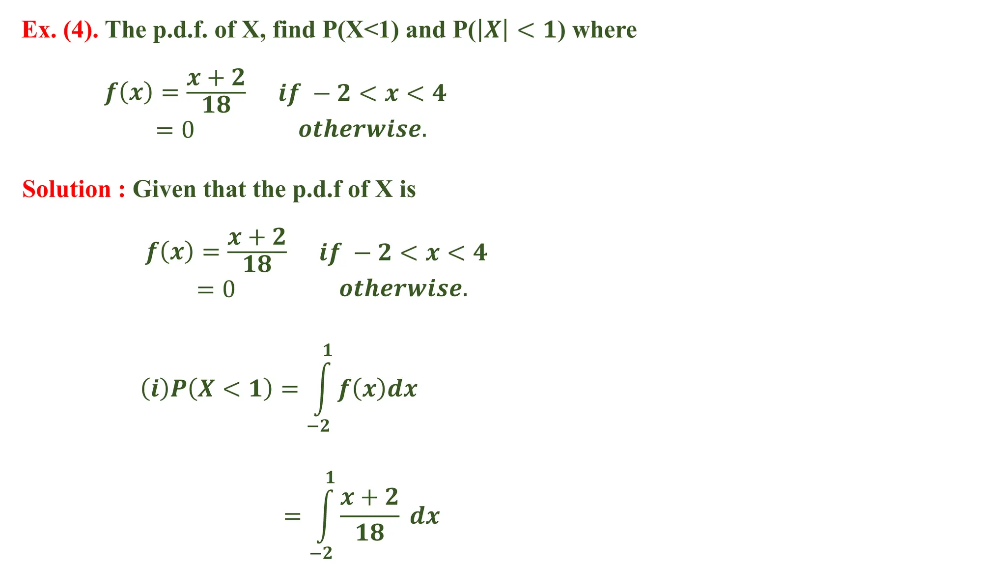
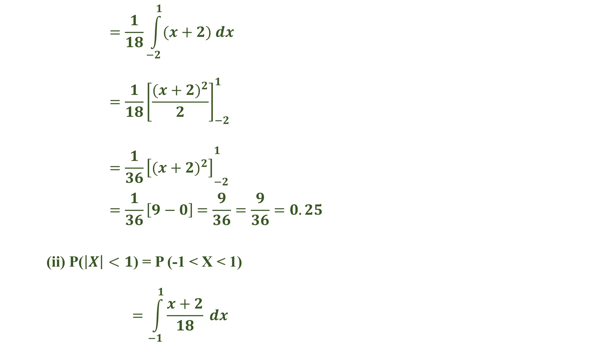
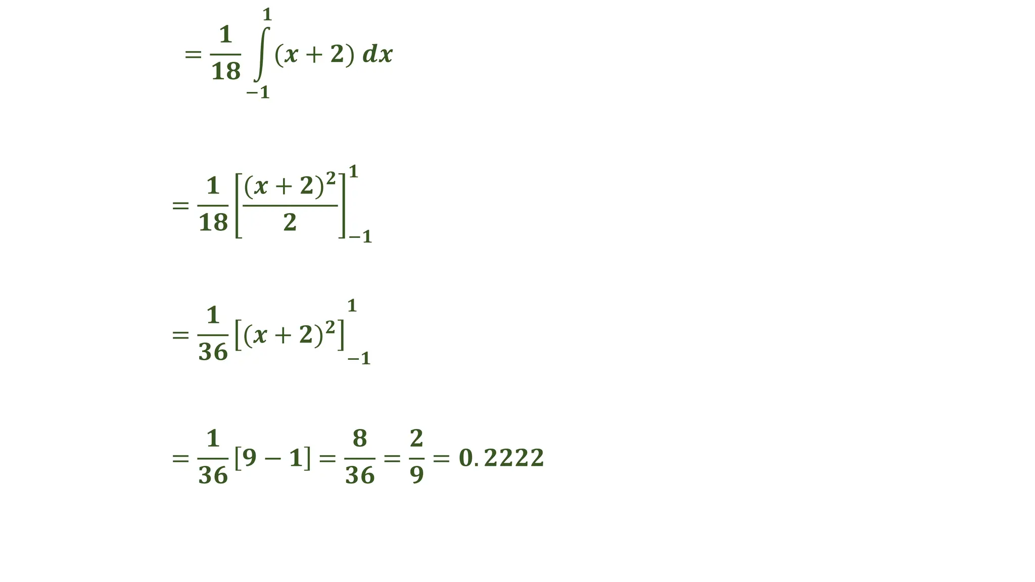
The document contains a series of examples related to probability distributions, including calculations of probabilities, expected values, variances, and standard deviations for various discrete random variables. It demonstrates how to derive parameters using given probability mass functions (pmfs) and probability density functions (pdfs). Additionally, it provides insights into calculating cumulative distributions and summaries of statistical properties for random variables.
![x𝒊 . p𝒊 𝟏
𝟔
𝟐
𝟔
𝟑
𝟔
𝟒
𝟔
𝟓
𝟔
𝟔
𝟔
𝟐𝟏
𝟔
=
𝟕
𝟐
𝒙𝒊
𝟐
. p𝒊
𝟏
𝟔
𝟒
𝟔
𝟗
𝟔
𝟏𝟔
𝟔
𝟐𝟓
𝟔
𝟑𝟔
𝟔
𝟗
𝟔
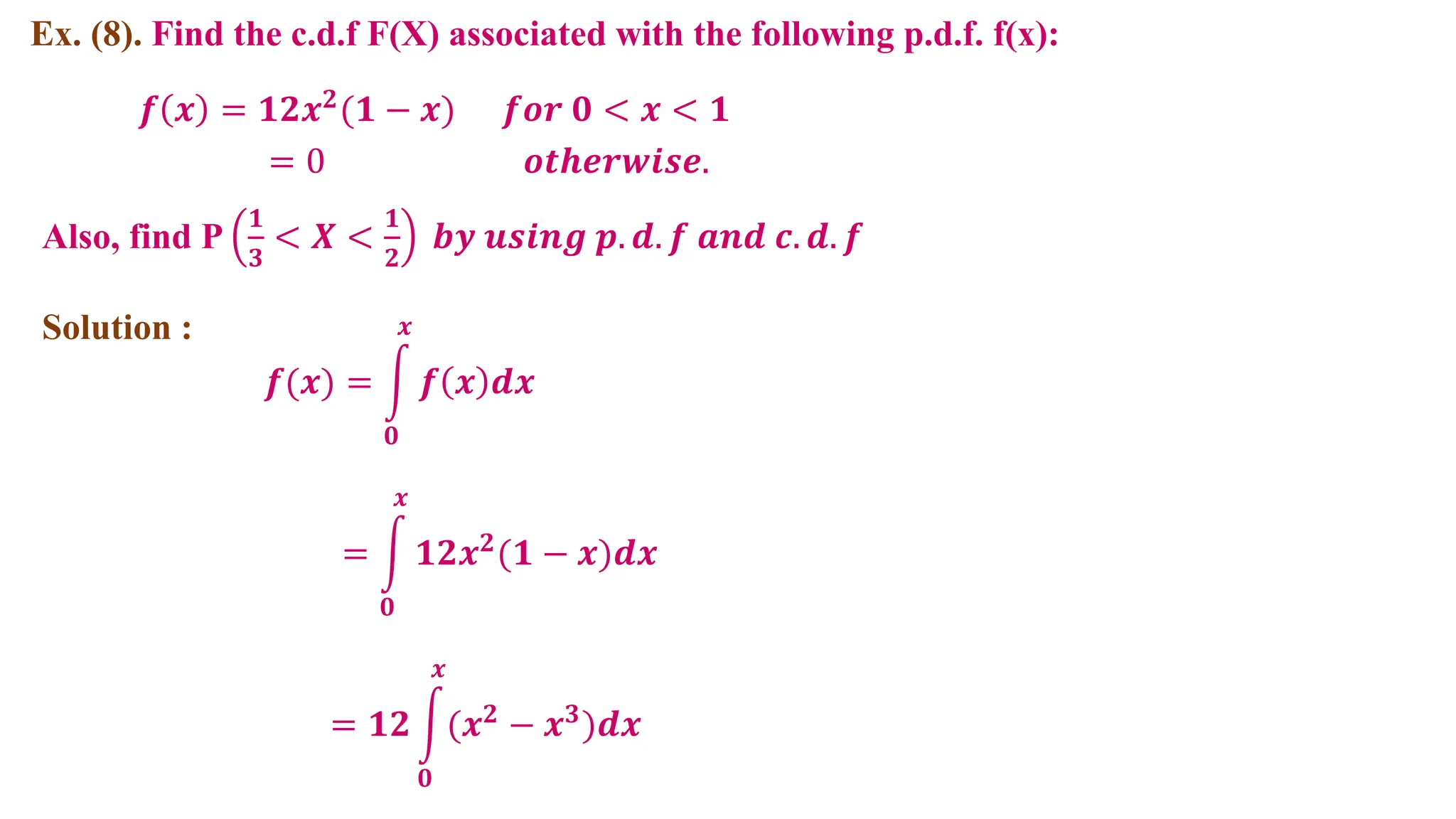
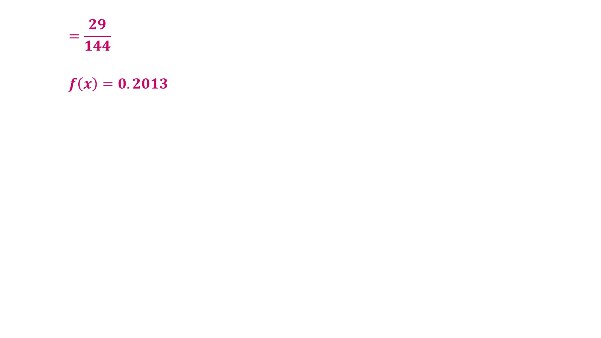
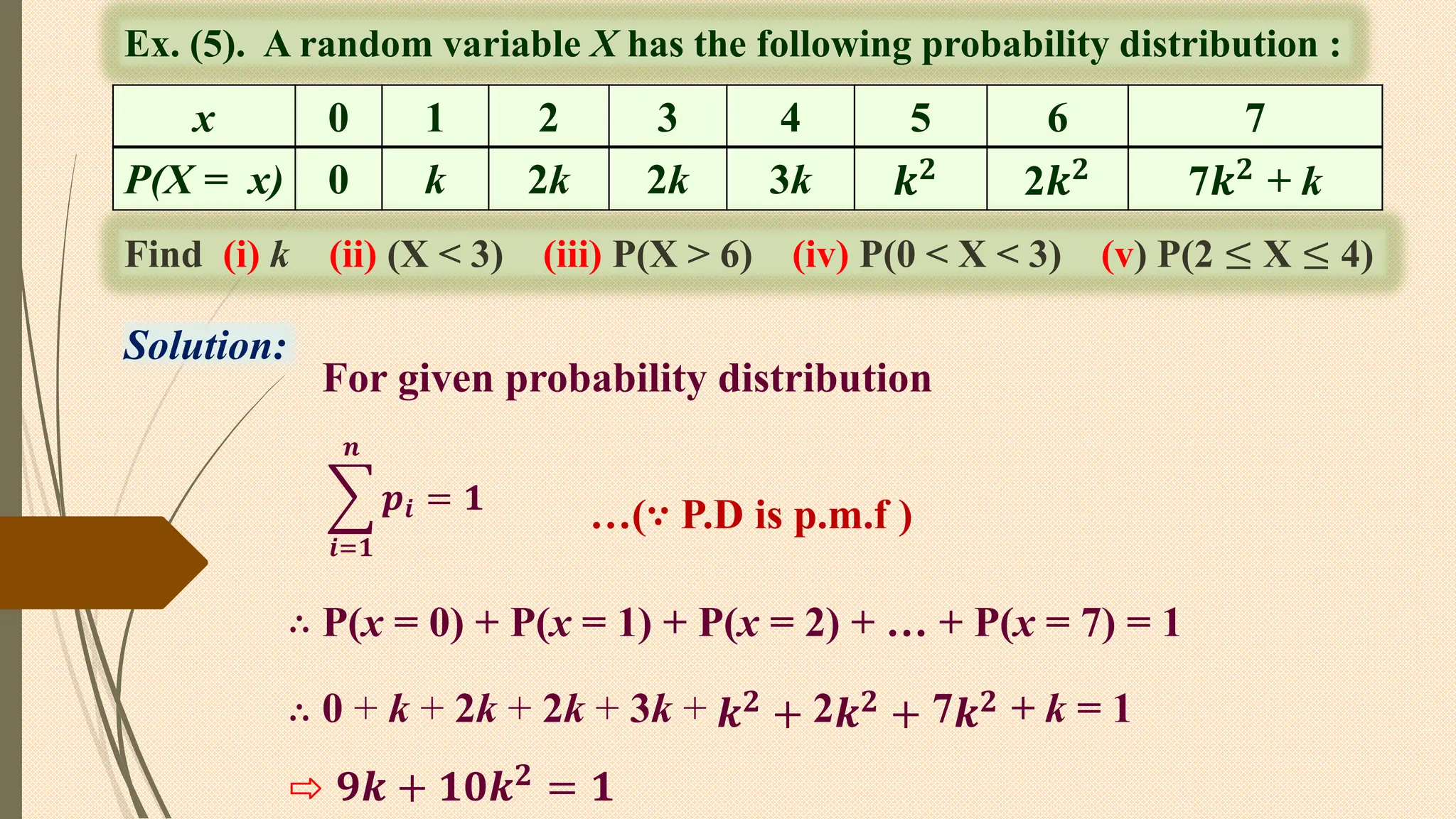
(i) Expected value = E(X) = 𝒙𝒊 , 𝒑𝒊 =
𝟕
𝟐
= 𝟑. 𝟓
𝒏
𝒊=𝟏
(ii) Variance = V(X) = E(𝑿𝟐) – [𝑬 𝑿 ]𝟐
𝒙𝒊
𝟐
, 𝒑𝒊 − 𝒙𝒊 , 𝒑𝒊
𝒏
𝒊=𝟏
𝟐
𝒏
𝒊=𝟏
=
𝟗𝟏
𝟔
−
𝟕
𝟐
𝟐
=
𝟗𝟏
𝟔
−
𝟒𝟗
𝟒
=
𝟏𝟖𝟐 − 𝟏𝟒𝟕
𝟏𝟐
∴ Variance =
𝟑𝟓
𝟏𝟐
= 𝟐. 𝟗𝟏𝟔𝟕](https://image.slidesharecdn.com/15probabilitydistributionpracticalhsc-240409193324-0beb7d55/75/15-Probability-Distribution-Practical-HSC-pdf-4-2048.jpg)
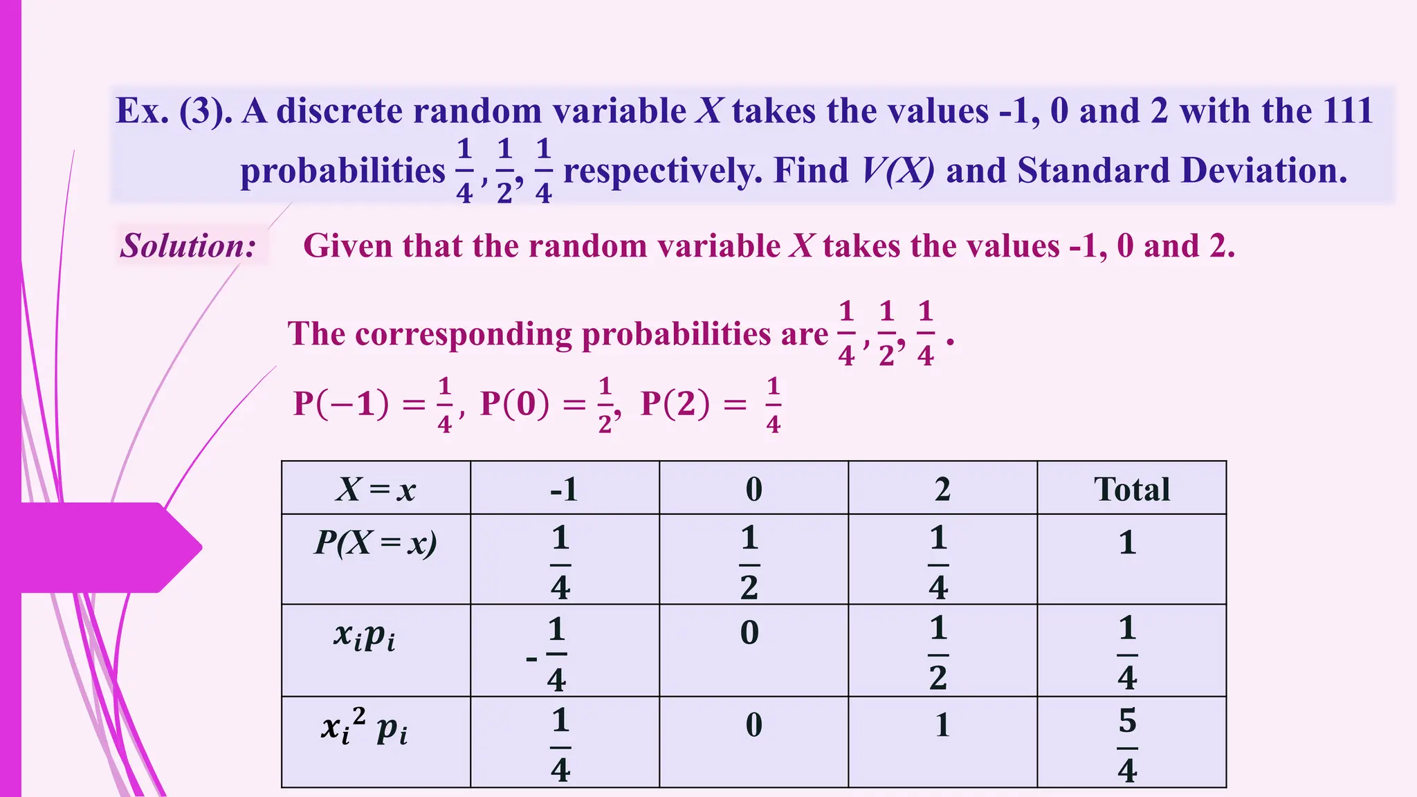
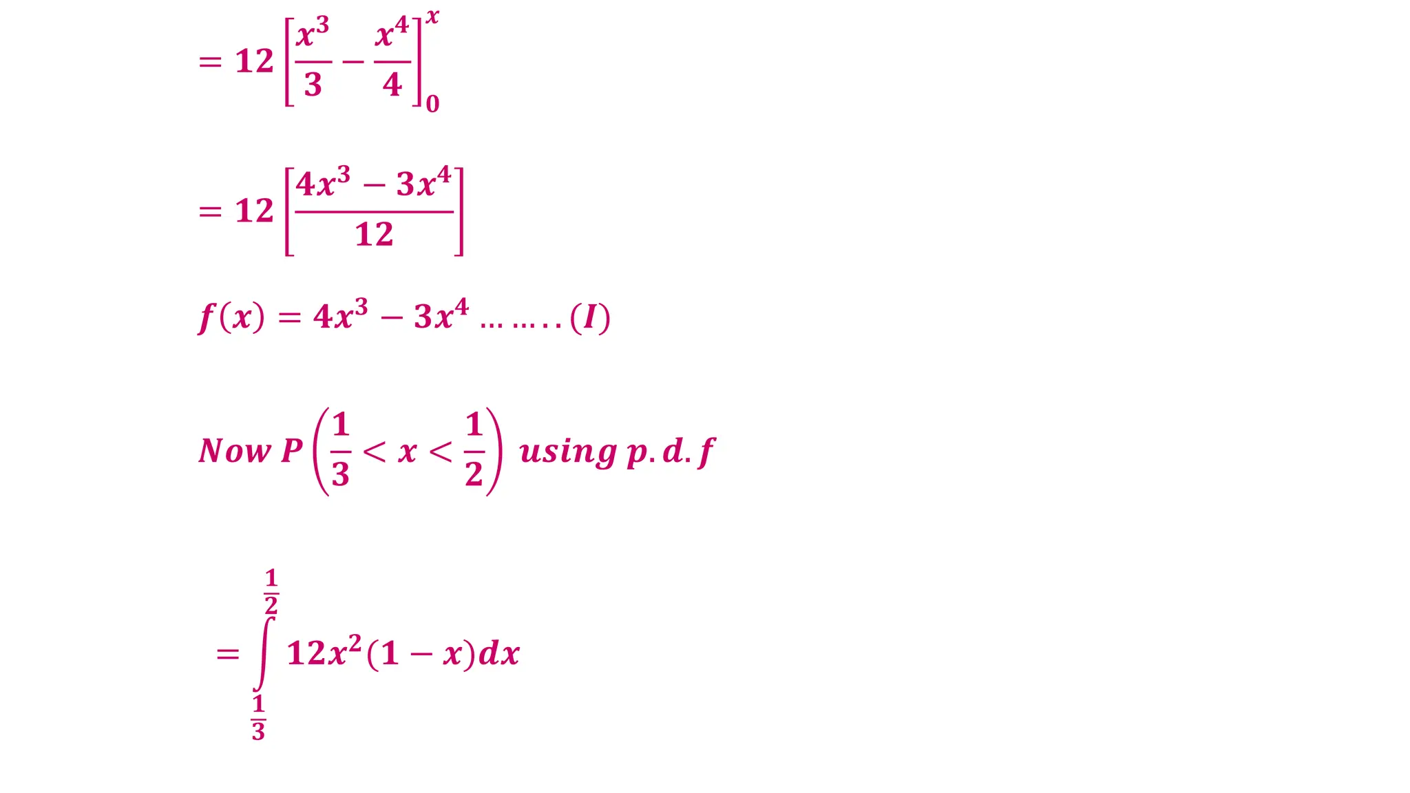
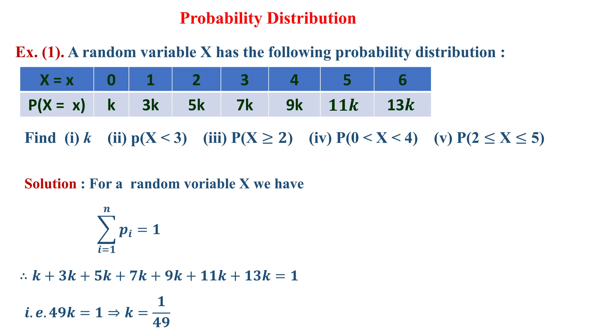
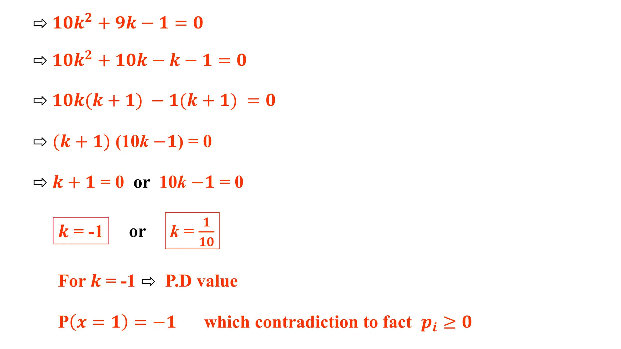
![(i) Variance = V(X) = E(𝑿𝟐) – [𝑬(𝑿)]𝟐
𝒙𝒊
𝟐 𝒑𝒊 −
𝒏
𝒊=𝟏
𝒙𝒊𝒑𝒊
𝒏
𝒊=𝟏
𝟐
=
𝟓
𝟒
−
𝟏
𝟒
𝟐
=
𝟓
𝟒
−
𝟏
𝟏𝟔
=
𝟓 × 𝟒 − 𝟏
𝟏𝟔
=
𝟐𝟎 − 𝟏
𝟏𝟔
=
𝟏𝟗
𝟏𝟔
= 1.1875
(ii) Standard Deviation = 𝝈 = V(X) =
𝟏𝟗
𝟏𝟔
= 𝟏. 𝟏𝟖𝟕𝟓 = 1.0897
Given data can be tabulated as follows (TABLE ON PREVIOUS PAGE )](https://image.slidesharecdn.com/15probabilitydistributionpracticalhsc-240409193324-0beb7d55/75/15-Probability-Distribution-Practical-HSC-pdf-6-2048.jpg)
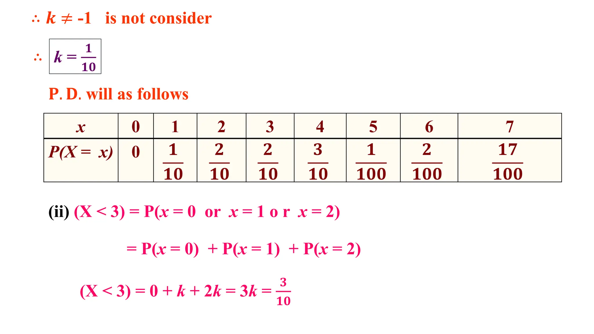
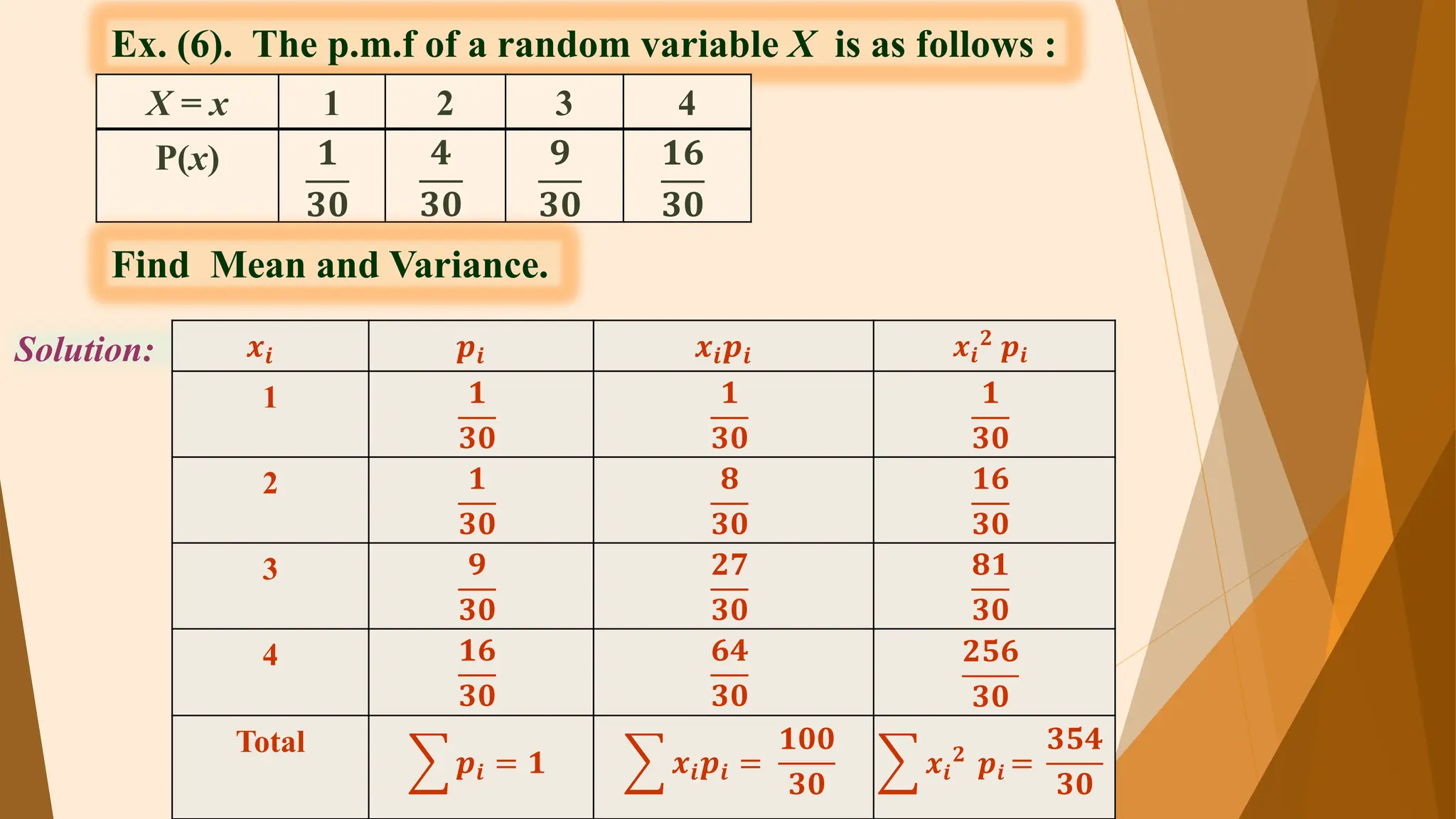
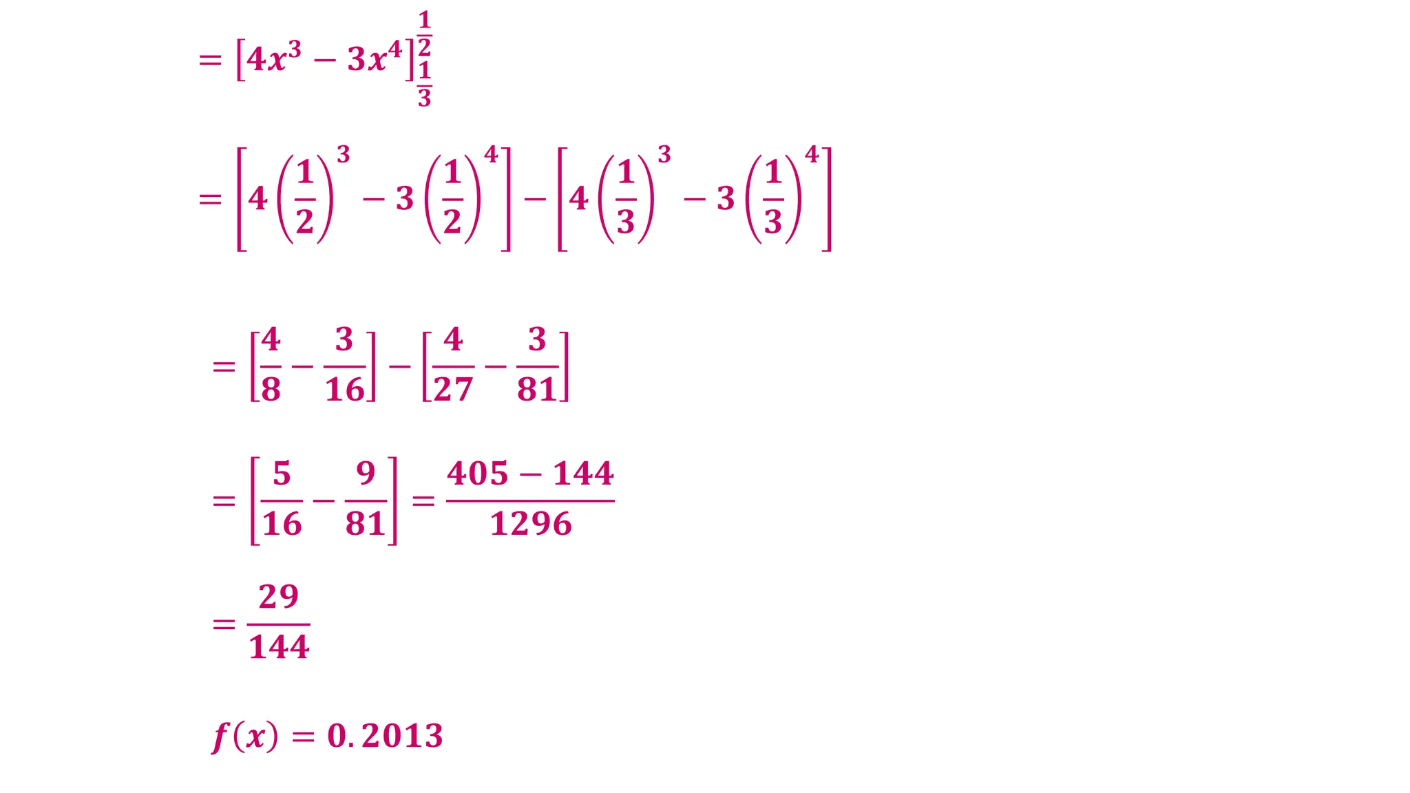
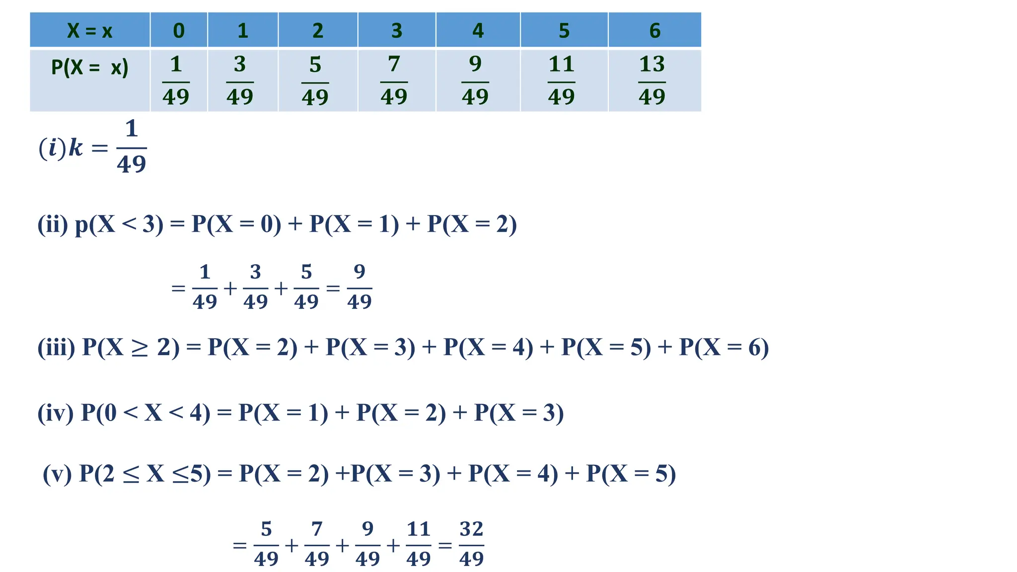
![Mean E(X) = 𝒙𝒊𝒑𝒊 =
𝟏𝟎𝟎
𝟑𝟎
𝒏
𝒊=𝟏
Mean =
𝟏𝟎𝟎
𝟑𝟎
Variance V(X) = E(𝑿𝟐
) - [𝐄(𝐗)]𝟐
= 𝒙𝒊
𝟐 𝒑𝒊 − 𝒙𝒊𝒑𝒊
𝒏
𝒊=𝟏
𝟐
𝒏
𝒊=𝟏
=
𝟑𝟓𝟒
𝟑𝟎
−
𝟏𝟎𝟎
𝟑𝟎
𝟐
=
𝟑𝟓𝟒
𝟑𝟎
−
𝟏𝟎,𝟎𝟎𝟎
𝟗𝟎𝟎
Variance =
𝟑𝟓𝟒 ×𝟑𝟎 − 𝟏𝟎,𝟎𝟎𝟎
𝟗𝟎𝟎
=
𝟏𝟖𝟔
𝟐𝟕𝟎
= 0.6888](https://image.slidesharecdn.com/15probabilitydistributionpracticalhsc-240409193324-0beb7d55/75/15-Probability-Distribution-Practical-HSC-pdf-15-2048.jpg)
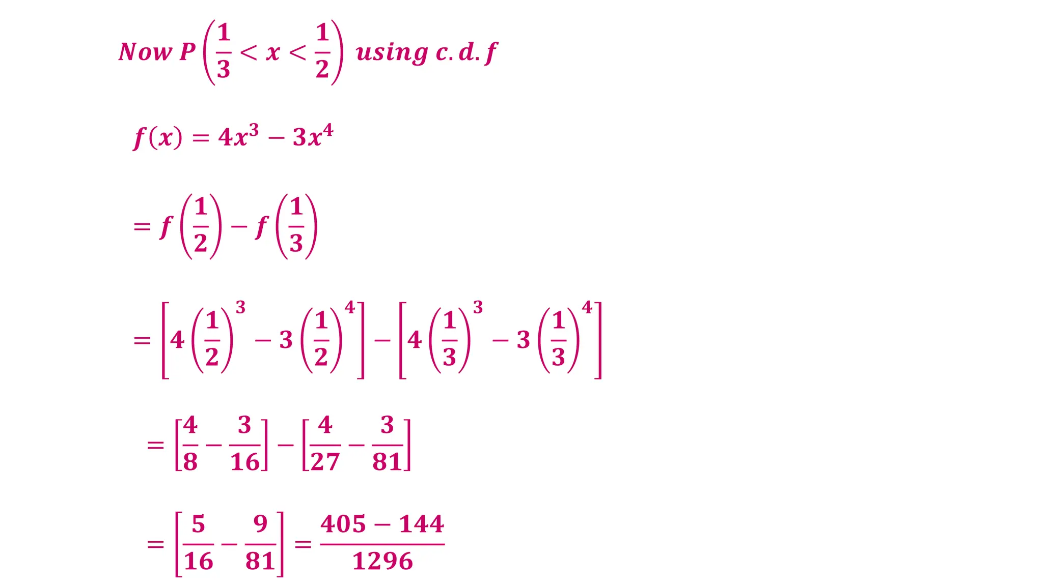
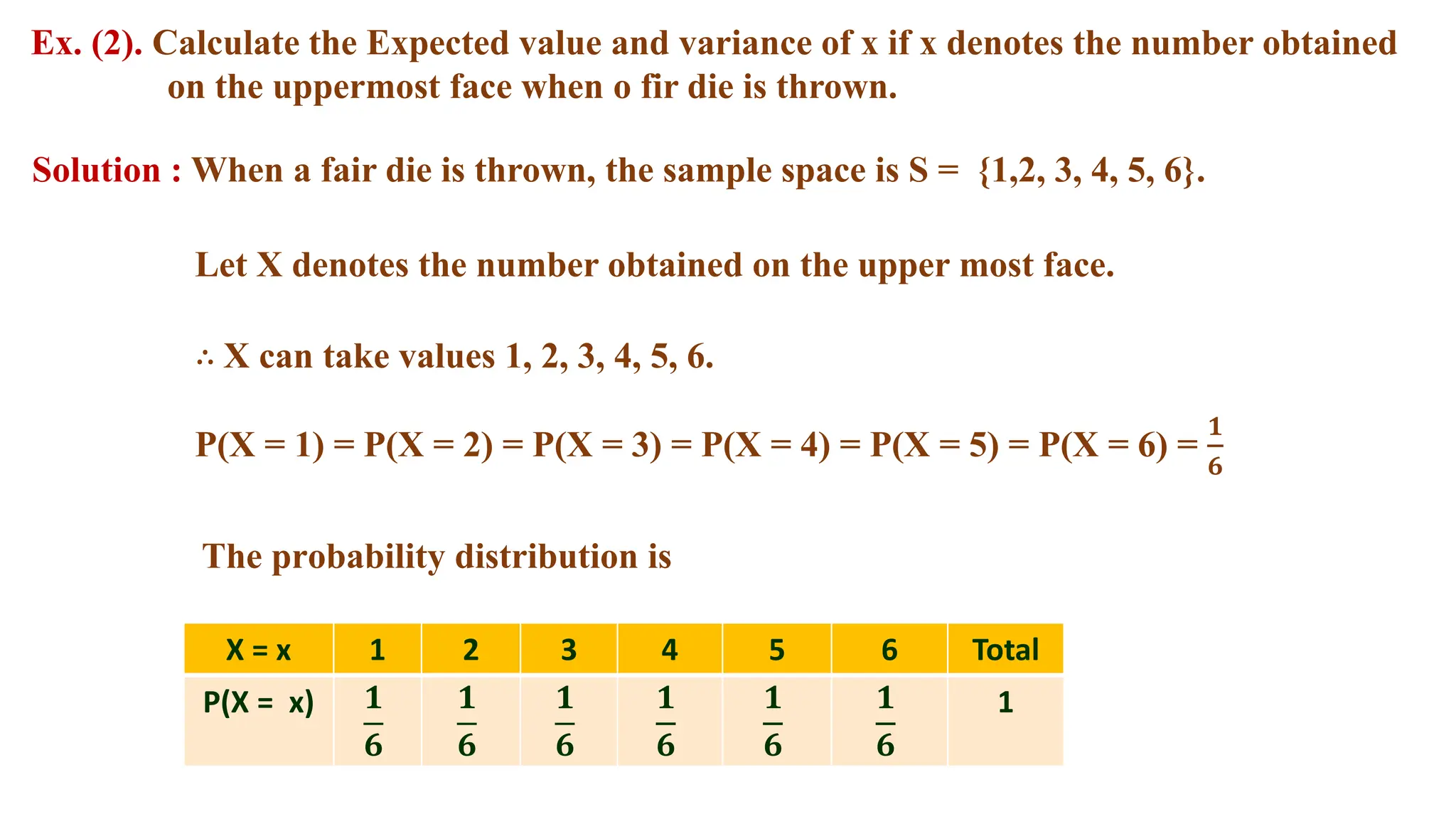
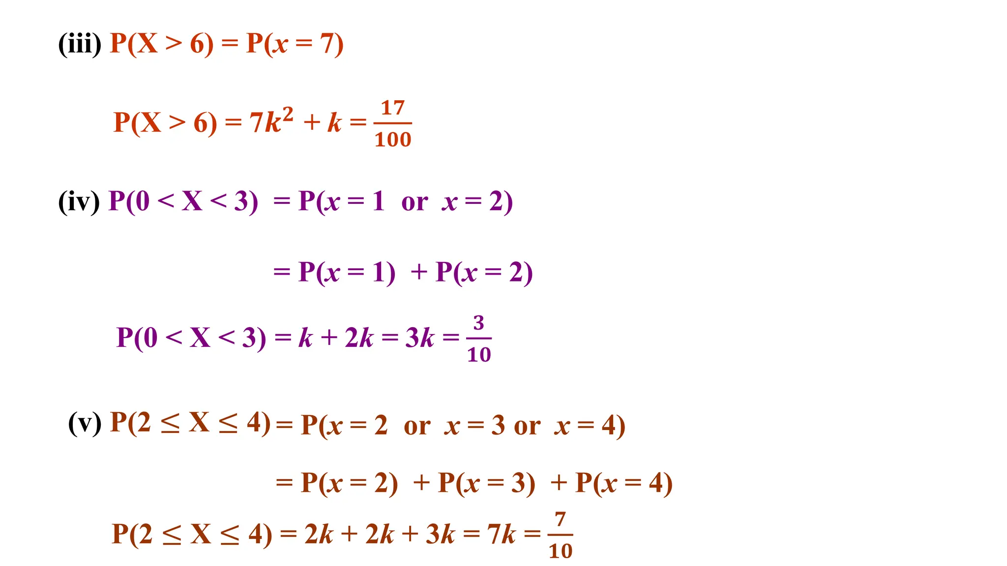
![Ex. (7). From a survey of 20 families in a society, the following data was obtained :
Solution:
No. of children 0 1 2 3 4
No. of families 𝟓 𝟏𝟏 𝟐 𝟎 2
For the random variable X = number of children in a randomly chosen family,
Find E(X) and V(X).
Total no. families = 5 + 11 + 2 + 0 + 2 = 20
X = { 0, 1, 2, 3, 4 }
Denotes random variable of no. children in a chosen family
P[x = 0] =
𝟓
𝟐𝟎
P[x = 1] =
𝟏𝟏
𝟐𝟎](https://image.slidesharecdn.com/15probabilitydistributionpracticalhsc-240409193324-0beb7d55/75/15-Probability-Distribution-Practical-HSC-pdf-16-2048.jpg)
![P[x = 2] =
𝟐
𝟐𝟎
, P[x = 3] =
𝟎
𝟐𝟎
and P[x = 4] =
𝟐
𝟐𝟎
𝒙𝒊 𝒑𝒊 𝒙𝒊𝒑𝒊 𝒙𝒊
𝟐 𝒑𝒊
0 𝟓
𝟐𝟎
𝟎 𝟎
1 𝟏𝟏
𝟐𝟎
𝟏𝟏
𝟐𝟎
𝟏𝟏
𝟐𝟎
2 𝟐
𝟐𝟎
𝟒
𝟐𝟎
𝟖
𝟐𝟎
3 𝟎
𝟐𝟎
= 0 𝟎 𝟎
4 𝟐
𝟐𝟎
𝟖
𝟐𝟎
𝟑𝟐
𝟐𝟎
Total
𝒑𝒊 = 𝟏 𝒙𝒊𝒑𝒊 =
𝟐𝟑
𝟐𝟎
𝒙𝒊
𝟐 𝒑𝒊 =
𝟓𝟏
𝟐𝟎](https://image.slidesharecdn.com/15probabilitydistributionpracticalhsc-240409193324-0beb7d55/75/15-Probability-Distribution-Practical-HSC-pdf-17-2048.jpg)
![Mean = E(X) = 𝒙𝒊𝒑𝒊 =
𝟐𝟑
𝟐𝟎
𝒏
𝒊=𝟏
Variance = V(X) = E(𝑿𝟐) - [𝐄(𝐗)]𝟐
= 𝒙𝒊
𝟐 𝒑𝒊 − 𝒙𝒊𝒑𝒊
𝒏
𝒊=𝟏
𝟐
𝒏
𝒊=𝟏
=
𝟓𝟏
𝟐𝟎
-
𝟐𝟑
𝟐𝟎
𝟐
=
𝟓𝟏 × 𝟐𝟎 − 𝟓𝟐𝟗
𝟒𝟎𝟎
Variance = V(X) =
𝟒𝟗𝟏
𝟒𝟎𝟎
= 𝟏. 𝟐𝟐𝟕𝟓](https://image.slidesharecdn.com/15probabilitydistributionpracticalhsc-240409193324-0beb7d55/75/15-Probability-Distribution-Practical-HSC-pdf-18-2048.jpg)