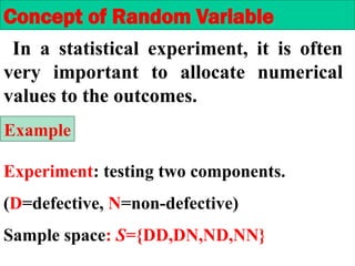
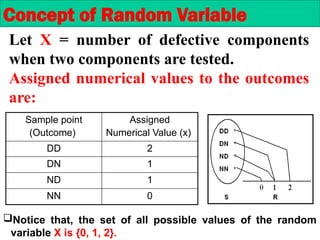
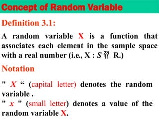
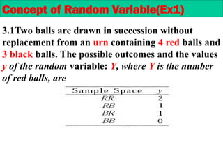
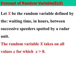
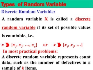
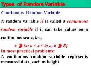
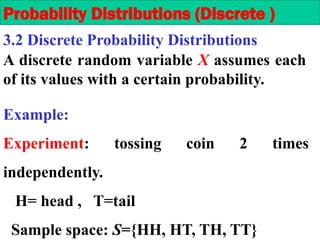
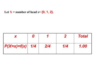
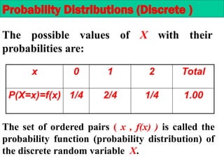
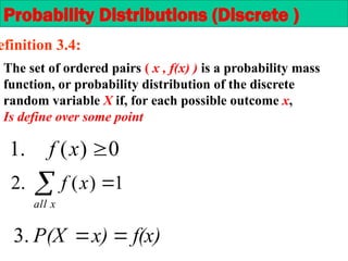
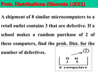
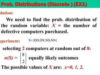
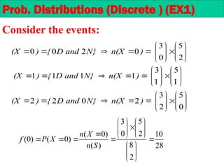
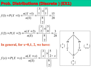
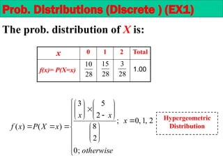
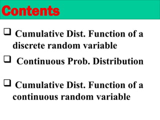
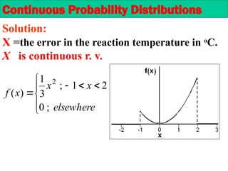
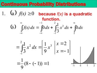
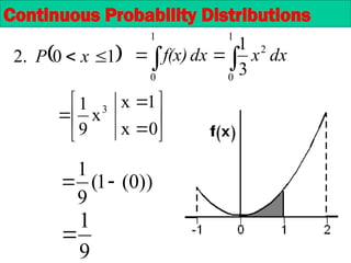
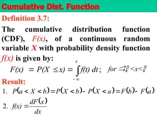
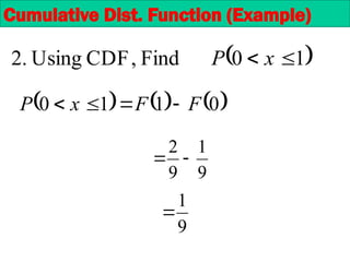
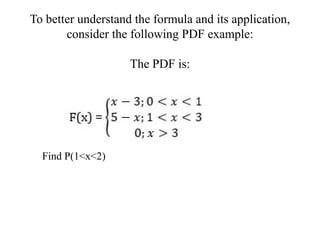
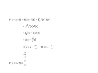
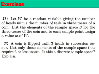
Lesson5 chapterfive Random Variable.pptx

‫جامعة‬
‫سويف‬ ‫بني‬
Probability and Statistics for Engineers

Random Variables and Probability
Distributions
Chapter 3

 Concept of Random Variable
Contents
 Discrete Probability Distribution

In a statistical experiment, it is often
very important to allocate numerical
values to the outcomes.
Experiment: testing two components.
(D=defective, N=non-defective)
Sample space: S={DD,DN,ND,NN}
Concept of Random Variable
Example

Let X = number of defective components
when two components are tested.
Assigned numerical values to the outcomes
are:
Sample point
(Outcome)
Assigned
Numerical Value (x)
DD 2
DN 1
ND 1
NN 0
Notice that, the set of all possible values of the random
variable X is {0, 1, 2}.

A random variable X is a function that
associates each element in the sample space
with a real number (i.e., X : S  R.)
" X “ (capital letter) denotes the random
variable .
" x " (small letter) denotes a value of the
random variable X.
Definition 3.1:
Notation

3.1Two balls are drawn in succession without
replacement from an urn containing 4 red balls and
3 black balls. The possible outcomes and the values
y of the random variable: Y, where Y is the number
of red balls, are
Concept of Random Variable(Ex1)

Let X be the random variable defined by
the: waiting time, in hours, between
successive speeders spotted by a radar
unit.
The random variable X takes on all
values x for which x > 0.
Concept of Random Variable(Ex2)

A random variable X is called a discrete
random variable if its set of possible values
is countable, i.e.,
x  {x1
, x2
, …, xn
} or x  {x1
, x2
, …}
In most practical problems:
A discrete random variable represents count
data, such as the number of defectives in a
sample of k items.
Types of Random Variable
Discrete Random Variable:

A random variable X is called a continuous
random variable if it can take values on a
continuous scale, i.e.,
x  {x: a < x < b; a, b  R}
In most practical problems:
A continuous random variable represents
measured data, such as height.
Types of Random Variable
Continuous Random Variable:

A discrete random variable X assumes each
of its values with a certain probability.
Example:
Experiment: tossing coin 2 times
independently.
H= head , T=tail
Sample space: S={HH, HT, TH, TT}
Probability Distributions (Discrete )
3.2 Discrete Probability Distributions

x 0 1 2 Total
P(X=x)=f(x) 1/4 2/4 1/4 1.00
Let X = number of head s= {0, 1, 2}.

The possible values of X with their
probabilities are:
x 0 1 2 Total
P(X=x)=f(x) 1/4 2/4 1/4 1.00
The set of ordered pairs ( x , f(x) ) is called the
probability function (probability distribution) of
the discrete random variable X.

1
)
(
.
2 
x
all
x
f
f(x)
x)
P(X 

3.
efinition 3.4:
0
)
(
.
1 
x
f
The set of ordered pairs ( x , f(x) ) is a probability mass
function, or probability distribution of the discrete
random variable X if, for each possible outcome x,
Is define over some point

Prob. Distributions (Discrete ) (EX1)
A shipment of 8 similar microcomputers to a
retail outlet contains 3 that are defective. If a
school makes a random purchase of 2 of
these computers, find the prob. Dist. for the
number of defectives.

We need to find the prob. distribution of
the random variable: X = the number of
defective computers purchased.
olution:
xperiment:
selecting 2 computers at random out of 8:
n(S) = equally likely outcomes








2
8
The possible values of X are: x=0, 1, 2.
S={DD,DN,ND,NN}

Consider the events:






















2
5
0
3
0
2
0
0 )
n(X
N}
D and
{
)
(X






















1
5
1
3
1
1
1
1 )
n(X
N}
D and
{
)
(X






















0
5
2
3
2
0
2
2 )
n(X
N}
D and
{
)
(X
28
10
2
8
2
5
0
3
)
(
)
0
(
)
0
(
)
0
( 






























S
n
X
n
X
P
f

28
15
2
8
1
5
1
3
)
(
)
1
(
)
1
(
)
1
( 






























S
n
X
n
X
P
f
28
3
2
8
0
5
2
3
)
(
)
2
(
)
2
(
)
2
( 






























S
n
X
n
X
P
f
In general, for x=0,1, 2, we have:































2
8
2
5
3
)
(
)
(
)
(
)
(
x
x
S
n
x
X
n
x
X
P
x
f

The prob. distribution of X is:
x 0 1 2 Total
f(x)= P(X=x)
28
10
28
15
28
3







































otherwise
x
x
x
x
X
P
x
f
;
0
2
,
1
,
0
;
2
8
2
5
3
)
(
)
(
Hypergeometric
Distribution
1.00

 Cumulative Dist. Function of a
discrete random variable
Contents
 Continuous Prob. Distribution
 Cumulative Dist. Function of a
continuous random variable

The cumulative dist. function (CDF), F(x),
of a discrete random variable X with the
probability function f(x) is given by:
;






x
t
f(t)
x)
P(X
F(x)
for <x<
Cumulative Distribution Function (CDF)
Definition 3.5:

Find the CDF of the random variable X with the
probability function if the pmf of X is:
x 0 1 2
f(x)
28
10
28
15
28
3
Cumulative Dist. Function (Ex 1)

F(x) = P(Xx) for <x<
For x<0 : F(x)=0
For 0x<1: F(x)=P(X=0)=
28
10
28
25
28
15
28
10


For 1x<2: F(x)=P(X=0)+P(X=1)=
For x2: F(x)=P(X=0)+P(X=1)
+P(X=2)
1
28
3
28
15
28
10




Solution:

The CDF of the random variable X is:


















2
;
1
2
1
;
28
25
1
0
;
28
10
0
;
0
)
(
)
(
x
x
x
x
x
X
P
x
F

F(0.5) = P(X0.5)=0
F(1.5)=P(X1.5)=F(1) =
F(3.8) =P(X3.8)=F(2)= 1
28
25
P(a < X  b) = P(X  b)  P(X  a) = F(b)  F(a)
P(a  X  b) = P(a < X  b) + P(X=a) = F(b)  F(a) + f(a)
P(a < X < b) = P(a < X  b)  P(X=b) = F(b)  F(a)  f(b)
Note:
Result:

Cumulative Dist. Function
• Example 3.10: Find the cumulative distribution function of
the random variable X in Example
• 3.9. Using F(x), Solution: Direct calculations of the
probability distribution of Example 3.9 give f(0)= 1/16,
• f(1) = 1/4, f(2)= 3/8, f(3)= 1/4, and f(4)= 1/16. Therefore,

Suppose that the probability function of X is:
x x1
x2
x3
… xn
F(x) f(x1
) f(x2
) f(x3
) … f(xn
)
Where x1
< x2
< … < xn
. Then:
F(xi
) = f(x1
) + f(x2
) + … + f(xi
) ; i=1, 2, …, n
F(xi
) = F(xi 1
) + f(xi
) ; i=2, …, n
f(xi
) = F(xi
)  F(xi 1
)
Result:

In the previous example,
28
15
28
10
28
25



28
3
28
25
1 


P(1 < X  2) = F(2)  F(1)
P(0.5 < X  1.5) = F(1.5)  F(0.5)

For any continuous random variable, X,
there exists a non-negative function f(x),
called the probability density function
(p.d.f) through which we can find
probabilities of events expressed in term
of X.
Continuous Probability Distributions

f: R  [0, )
= area under the curve
of f(x) and over the
region A
  



b
a
dx
f(x)
b
X
a
P
  


A
dx
f(x)
A
X
p
= area under the curve
of f(x) and over the interval
(a,b)

1
.
2 



-
dx
f(x)
Definition 3.6:
The function f(x) is a probability density
function (pdf) for a continuous random
variable X, defined on the set of real
numbers, if:
  



b
a
dx
f(x)
b
X
a
P
.
3  a, b  R ; a  b
R
x
f(x) 

0
.
1

P(a  X  b)= P(a < X  b)
= P(a  X < b)
= P(a < X < b)
Note:
We shall concern ourselves with computing
prob. for various intervals of continuous
random variables such as P(a < X < b),
P(W > c), and so forth.
Note that when X is continuous,

 
 





b
a
dx
x
f
b
X
a
P
area
 
 





b
dx
x
f
b
X
P
area  
 





a
dx
x
f
a
X
P
area
  1


 



dx
x
f
area
Total

Suppose that the error in the reaction temperature, in o
C,
for a controlled laboratory experiment is a continuous
random variable X having the following probability
density function:









elsewhere
x
x
x
f
;
0
2
1
;
3
1
)
(
2
  1




-
dx
f(x)
b
Example 3.6:
  0
a
t
Verify tha
.
1 
f(x)
 
1
0
Find
.
2 
 x
P

Solution:
X =the error in the reaction temperature in o
C.
X is continuous r. v.









elsewhere
x
x
x
f
;
0
2
1
;
3
1
)
(
2

because f(x) is a quadratic
function.
  











2
2
1
2
1
0
3
1
0 dx
dx
x
dx
dx
f(x)
b
-
-
-










 1
2
9
1
3
1 3
2
1
2
x
x
x
dx
x
-
1
))
1
(
8
(
9
1




  0
a
1. 
f(x)


 

1
0
2
1
0
3
1
dx
x
dx
f(x)









0
x
1
x
x
9
1 3
))
0
(
1
(
9
1


9
1

 
1
0
.
2 
 x
P

The cumulative distribution function
(CDF), F(x), of a continuous random
variable X with probability density function
f(x) is given by:
Definition 3.7:
;







x
dt
f(t)
x)
P(X
F(x) for  <x<
Result:
         
 
dx
x
dF
f(x)
a
F
b
F
a
X
P
b
X
P
b
X
a
P









.
2
.
1

Suppose that the error in the reaction temperature, in o
C,
for a controlled laboratory experiment is a continuous
random variable X having the following probability
density function:









elsewhere
x
x
x
f
;
0
2
1
;
3
1
)
(
2
Example 3.6:
CDF
the
Find
.
1
 
1
0
Find
,
CDF
Using
.
2 
 x
P
Cumulative Dist. Function (Example)
P(1 X 2)
˂ ˂

Solution:









elsewhere
x
x
x
f
;
0
2
1
;
3
1
)
(
2
  0
0
1
For






 

x
-
x
-
dt
dt
f(t)
x
F
x
  

 







x
-
-
x
-
dt
t
dt
dt
f(t)
x
F
x
1
2
1
3
1
0
2
1
-
For


x
-
dt
t
1
2
3
1

)
1
(
9
1
))
1
(
(
9
1
1
9
1 3
3
3














 x
x
t
x
t
t
  

 







x
-
-
x
-
dt
t
dt
dt
f(t)
x
F
x
1
2
1
3
1
0
2
1
-
For


x
-
dt
t
1
2
3
1
  =
dt
dt
t
dt
dt
f(t)
x
F
x
x
-
-
x
-



 






 2
2
1
2
1
0
3
1
0
2
For
1
3
1
2
1
2


-
dt
t

Therefore, the CDF is:

















2
;
1
2
1
;
)
1
(
9
1
1
;
0
)
(
)
( 3
x
x
x
x
x
X
P
x
F

9
1
9
2


 
1
0
Find
,
CDF
Using
.
2 
 x
P
     
0
1
1
0 F
F
x
P 



9
1


To better understand the formula and its application,
consider the following PDF example:
The PDF is:
Find P(1<x<2)

Lesson5 chapterfive Random Variable.pptx

More Related Content

Similar to Lesson5 chapterfive Random Variable.pptx

More from hebaelkouly

Recently uploaded

Lesson5 chapterfive Random Variable.pptx